ZMA Sleep Experiment
A randomized blinded self-experiment of the effects of ZMA (zinc+magnesium+vitamin B6) on my sleep; results suggest small benefit to sleep quality but are underpowered and damaged by Zeo measurement error/data issues.
I ran a blinded randomized self-experiment of 2.5g nightly ZMA powder effect on Zeo-recorded sleep data during March-October 2017 (n = 127). The linear model and SEM model show no statistically-significant effects or high posterior probability of benefits, although all point-estimates were in the direction of benefits. Data quality issues reduced the available dataset, rendering the experiment particularly underpowered and the results more inconclusive. I decided to not continue use of ZMA after running out; ZMA may help my sleep but I need to improve data quality before attempting any further sleep self-experiments on it.
The supplement “ZMA” (short for “Zinc Magnesium Aspartate”; Examine) is a supplement mix of zinc, magnesium and vitamin B6. The combination is semi-popular for athletes/weight-lifters but it’s also commonly said to be good for sleep, perhaps due to the magnesium. I haven’t looked at the research literature on it too closely, of which there is not much, but come on - how harmful could zinc, magnesium, or vitamin B6 be? Seemed worth a shot, and more than one person has asked me about it. So testing ZMA has for a long time been a (low) priority in my sleep experiments.
Background
In March 2017, nootropics website Powder City announced a going-out-of-business sale (speculated to be due to a wrongful-death lawsuit over a guy who decided to commit suicide using tianeptine, which was eventually settled); I took advantage of it to pick up caffeine, theanine, sulbutiamine, creatine and, since some other things I wanted had sold out, picked up 200g of ZMA powder for a total of $25.98$19.272017 (after coupon & shipping).
The suggested dose is ~2.5g⧸day (3 1cc scoops), with the contents listed as follows:
Vitamin B6 as Pyridoxine Hydrochloride: 10.5mg
Magnesium as aspartate: 250mg
Zinc as mono-l-methionine and aspartate: 30mg
So my 200g / 2.5g = 80 doses or 19.27 / 80 = $0.32$0.242017 per dose (or ~$121.34$902017/year).
Because of my bad experience with potassium, I didn’t jump straight into a blinded self-experiment but I briefly used ZMA as directed before bedtime 22-2017-03-27. I didn’t notice anything bad or good (if ZMA does cause “weird dreams”, it apparently did not do anything noticeable for me beyond what melatonin) so I continued.
Design
ZMA doesn’t require anything special for a blinded self-experiment, as it’s a normal white powder without an overwhelming taste, so it can be simply capped. I took the remaining 185g/75 doses and capped 216 ZMA pills (24x9 batches); I capped a corresponding 240 flour pills. Total time capping & cleaning: 2h - ZMA powder, like magnesium citrate powder, is a pain to cap because it is a fluffy sticky powder which eventually starts to jam the pill machine, requiring it to be washed and thoroughly dried before doing a second batch.
With 185g turning into 216 pills, that implies ~0.86g/pill, requiring 3 pills to reach the target dose of ~2.57g; at 3 pills per night, 72 nights of ZMA or 144 days total.
For simplicity I went with my usual blinding & randomization method of paired-days / paired-jars. Because my sample size is limited by how much ZMA I had on hand, I did not do any power analysis.
The experiment ran from 2017-03-30 to 2017-10-09. I ran into two major issues: there were a large number of interruptions due to forgetting or travel (eg. a meditation retreat) or other issues, and my Zeo data quality appears to be declining considerably, with both missing-nights increasing & ZQ dropping improbably much (perhaps because my last headband is wearing out or due to subtle electrical-wiring issues again screwing with voltage) - that or my sleep really did degrade that drastically over 2016–2017. As well, my previous magnesium experiments suggest there are cumulative long-term effects of magnesium supplementation which blocking pairs of days would hide, but I haven’t confirmed this and discussions of ZMA/sleep claim acute benefits. Between these problems, I am unhappy with how the experiment’s quality turned out: the sample size was too low to start with, the Zeo data issues decreased it further with noisier & missing data, and the causal interpretation is a little shaky.
Analysis
Description
zma <- read.csv("https://gwern.net/doc/zeo/2018-01-04-zeo-zma.csv", colClasses=c("Date", rep("integer", 11)))
summary(zma)
#       Date                  ZQ               Total.Z           Time.to.Z         Time.in.Wake        Time.in.REM
#  Min.   :2017-03-30   Min.   :  1.00000   Min.   : 20.0000   Min.   : 1.00000   Min.   :  0.00000   Min.   :  1.00000
#  1st Qu.:2017-05-15   1st Qu.: 44.00000   1st Qu.:288.0000   1st Qu.: 2.00000   1st Qu.:  3.00000   1st Qu.: 36.00000
#  Median :2017-07-04   Median : 64.00000   Median :382.0000   Median : 3.00000   Median : 11.00000   Median : 77.00000
#  Mean   :2017-07-03   Mean   : 60.98758   Mean   :369.1801   Mean   : 7.78882   Mean   : 19.54658   Mean   : 76.19255
#  3rd Qu.:2017-08-21   3rd Qu.: 80.00000   3rd Qu.:473.0000   3rd Qu.:11.00000   3rd Qu.: 27.00000   3rd Qu.:111.00000
#  Max.   :2017-10-09   Max.   :102.00000   Max.   :588.0000   Max.   :41.00000   Max.   :121.00000   Max.   :184.00000
#                       NA's   :38          NA's   :38         NA's   :38         NA's   :38          NA's   :38
#  Time.in.Light       Time.in.Deep        Awakenings          Rise.Time         Morning.Feel           ZMA
#  Min.   : 18.0000   Min.   : 1.00000   Min.   : 0.000000   Min.   :346.0000   Min.   :0.000000   Min.   :0.0000000
#  1st Qu.:218.0000   1st Qu.:20.00000   1st Qu.: 2.000000   1st Qu.:526.0000   1st Qu.:2.000000   1st Qu.:0.0000000
#  Median :274.0000   Median :35.00000   Median : 4.000000   Median :566.0000   Median :2.000000   Median :0.0000000
#  Mean   :258.4783   Mean   :35.01242   Mean   : 4.776398   Mean   :559.4472   Mean   :2.173913   Mean   :0.4932432
#  3rd Qu.:328.0000   3rd Qu.:47.00000   3rd Qu.: 7.000000   3rd Qu.:596.0000   3rd Qu.:3.000000   3rd Qu.:1.0000000
#  Max.   :422.0000   Max.   :96.00000   Max.   :13.000000   Max.   :811.0000   Max.   :3.000000   Max.   :1.0000000
#  NA's   :38         NA's   :38         NA's   :38          NA's   :38         NA's   :38         NA's   :51
round(digits=2, cor(zma[,-1], use="pairwise.complete.obs"))
#                  ZQ Total.Z Time.to.Z Time.in.Wake Time.in.REM Time.in.Light Time.in.Deep Awakenings Rise.Time Morning.Feel   ZMA
# ZQ             1.00
# Total.Z        0.98    1.00
# Time.to.Z      0.22    0.24      1.00
# Time.in.Wake  -0.24   -0.08      0.14         1.00
# Time.in.REM    0.73    0.76      0.34         0.04        1.00
# Time.in.Light  0.91    0.95      0.14        -0.06        0.54          1.00
# Time.in.Deep   0.77    0.67      0.14        -0.36        0.30          0.62         1.00
# Awakenings     0.23    0.37      0.39         0.59        0.53          0.27        -0.02       1.00
# Rise.Time      0.31    0.30     -0.16        -0.09        0.12          0.32         0.27      -0.05      1.00
# Morning.Feel   0.23    0.25     -0.09        -0.03        0.21          0.25         0.07       0.07      0.13         1.00
# ZMA            0.10    0.07     -0.04        -0.08        0.14          0.02         0.08      -0.10      0.07        -0.04  1.00
library(gridExtra); library(ggplot2)
p1 <- qplot(Date, Time.to.Z,     color=ZMA, data=zma) + stat_smooth(se=FALSE) + theme(legend.position = "none", axis.title.x=element_blank())
p2 <- qplot(Date, Time.in.Wake,  color=ZMA, data=zma) + stat_smooth(se=FALSE) + theme(legend.position = "none", axis.title.x=element_blank())
p3 <- qplot(Date, Time.in.Light, color=ZMA, data=zma) + stat_smooth(se=FALSE) + theme(legend.position = "none", axis.title.x=element_blank())
p4 <- qplot(Date, Time.in.REM,   color=ZMA, data=zma) + stat_smooth(se=FALSE) + theme(legend.position = "none", axis.title.x=element_blank())
p5 <- qplot(Date, Time.in.Deep,  color=ZMA, data=zma) + stat_smooth(se=FALSE) + theme(legend.position = "none", axis.title.x=element_blank())
p6 <- qplot(Date, Total.Z,       color=ZMA, data=zma) + stat_smooth(se=FALSE) + theme(legend.position = "none", axis.title.x=element_blank())
p7 <- qplot(Date, Awakenings,    color=ZMA, data=zma) + stat_smooth(se=FALSE) + theme(legend.position = "none", axis.title.x=element_blank())
p8 <- qplot(Date, Rise.Time,     color=ZMA, data=zma) + stat_smooth(se=FALSE) + theme(legend.position = "none", axis.title.x=element_blank())
p9 <- qplot(Date, Morning.Feel,  color=ZMA, data=zma) + stat_smooth(se=FALSE) + theme(legend.position = "none", axis.title.x=element_blank())
grid.arrange(p1, p2, p3, p4, p5, p6, p7, p8, p9, ncol=2)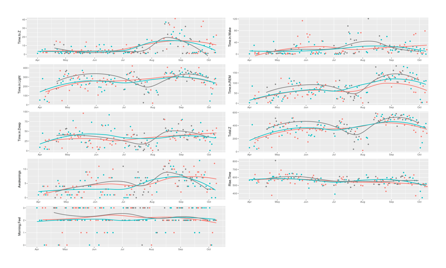
9 Zeo sleep variables plotted over the course of the ZMA supplement sleep self-experiment
Modeling
The usual simple-minded linear model:
l <- lm(cbind(ZQ, Total.Z, Time.to.Z, Time.in.Wake, Time.in.REM, Time.in.Light, Time.in.Deep, Awakenings, Rise.Time,
              Morning.Feel) ~ ZMA, data=zma); summary(l)
# Response ZQ :
# Coefficients:
#              Estimate Std. Error  t value Pr(>|t|)
# (Intercept) 57.692308   2.882334 20.01583  < 2e-16
# ZMA          4.839950   4.125251  1.17325  0.24293
#
# Residual standard error: 23.23812 on 125 degrees of freedom
#   (72 observations deleted due to missingness)
# Multiple R-squared:  0.01089218,  Adjusted R-squared:  0.002979316
# F-statistic: 1.376516 on 1 and 125 DF,  p-value: 0.2429264
#
# Response Total.Z :
# Coefficients:
#              Estimate Std. Error  t value Pr(>|t|)
# (Intercept) 353.47692   16.12152 21.92578  < 2e-16
# ZMA          19.08759   23.07342  0.82725  0.40967
#
# Residual standard error: 129.9759 on 125 degrees of freedom
#   (72 observations deleted due to missingness)
# Multiple R-squared:  0.00544499,  Adjusted R-squared:  -0.00251145
# F-statistic:  0.68435 on 1 and 125 DF,  p-value: 0.4096693
#
# Response Time.to.Z :
# Coefficients:
#               Estimate Std. Error  t value   Pr(>|t|)
# (Intercept)  8.0000000  1.1118491  7.19522 5.0703e-11
# ZMA         -0.6451613  1.5912993 -0.40543    0.68585
#
# Residual standard error: 8.964014 on 125 degrees of freedom
#   (72 observations deleted due to missingness)
# Multiple R-squared:  0.001313264, Adjusted R-squared:  -0.00667623
# F-statistic: 0.1643739 on 1 and 125 DF,  p-value: 0.6858542
#
# Response Time.in.Wake :
# Coefficients:
#              Estimate Std. Error  t value   Pr(>|t|)
# (Intercept) 19.615385   2.683811  7.30878 2.8102e-11
# ZMA         -3.470223   3.841120 -0.90344    0.36803
#
# Residual standard error: 21.63757 on 125 degrees of freedom
#   (72 observations deleted due to missingness)
# Multiple R-squared:  0.006487277, Adjusted R-squared:  -0.001460825
# F-statistic: 0.8162046 on 1 and 125 DF,  p-value: 0.36803
#
# Response Time.in.REM :
# Coefficients:
#              Estimate Std. Error  t value Pr(>|t|)
# (Intercept) 66.184615   5.562789 11.89774  < 2e-16
# ZMA         12.379901   7.961568  1.55496  0.12248
#
# Residual standard error: 44.84864 on 125 degrees of freedom
#   (72 observations deleted due to missingness)
# Multiple R-squared:  0.01897609,  Adjusted R-squared:  0.0111279
# F-statistic: 2.417893 on 1 and 125 DF,  p-value: 0.1224844
#
# Response Time.in.Light :
# Coefficients:
#               Estimate Std. Error  t value Pr(>|t|)
# (Intercept) 254.123077  10.926307 23.25791  < 2e-16
# ZMA           3.554342  15.637936  0.22729  0.82057
#
# Residual standard error: 88.09071 on 125 degrees of freedom
#   (72 observations deleted due to missingness)
# Multiple R-squared:  0.0004131143,    Adjusted R-squared:  -0.007583581
# F-statistic: 0.05166063 on 1 and 125 DF,  p-value: 0.8205698
#
# Response Time.in.Deep :
# Coefficients:
#              Estimate Std. Error  t value Pr(>|t|)
# (Intercept) 33.707692   2.495414 13.50785  < 2e-16
# ZMA          3.098759   3.571484  0.86764  0.38725
#
# Residual standard error: 20.11867 on 125 degrees of freedom
#   (72 observations deleted due to missingness)
# Multiple R-squared:  0.005986331, Adjusted R-squared:  -0.001965779
# F-statistic: 0.7527978 on 1 and 125 DF,  p-value: 0.3872545
#
# Response Awakenings :
# Coefficients:
#               Estimate Std. Error  t value Pr(>|t|)
# (Intercept)  4.9384615  0.4312593 11.45126  < 2e-16
# ZMA         -0.6965261  0.6172264 -1.12848  0.26128
#
# Residual standard error: 3.476924 on 125 degrees of freedom
#   (72 observations deleted due to missingness)
# Multiple R-squared:  0.01008495,  Adjusted R-squared:  0.002165627
# F-statistic: 1.273461 on 1 and 125 DF,  p-value: 0.2612796
#
# Response Rise.Time :
# Coefficients:
#               Estimate Std. Error  t value Pr(>|t|)
# (Intercept) 555.230769   7.176394 77.36905  < 2e-16
# ZMA           7.946650  10.270989  0.77370  0.44057
#
# Residual standard error: 57.85794 on 125 degrees of freedom
#   (72 observations deleted due to missingness)
# Multiple R-squared:  0.004766052, Adjusted R-squared:  -0.003195819
# F-statistic: 0.5986096 on 1 and 125 DF,  p-value: 0.4405698
#
# Response Morning.Feel :
# Coefficients:
#                Estimate  Std. Error  t value Pr(>|t|)
# (Intercept)  2.16923077  0.11124903 19.49887  < 2e-16
# ZMA         -0.07245658  0.15922170 -0.45507  0.64985
#
# Residual standard error: 0.8969184 on 125 degrees of freedom
#   (72 observations deleted due to missingness)
# Multiple R-squared:  0.001653949, Adjusted R-squared:  -0.006332819
# F-statistic: 0.2070862 on 1 and 125 DF,  p-value: 0.6498503
summary(manova(l))
#            Df      Pillai   approx F num Df den Df  Pr(>F)
# ZMA         1 0.087584221 0.91191989     12    114 0.53755
# Residuals 125
# Table:
Variable |
Effect |
p-value |
Better |
|---|---|---|---|
ZQ |
4.84 |
0.24 |
Yes |
Total Z |
19.1 |
0.41 |
Yes |
Time to Z |
-0.65 |
0.69 |
Yes |
Time in Wake |
-3.47 |
0.37 |
Yes |
Time in REM |
12.38 |
0.12 |
Yes |
Time in Light |
3.55 |
0.82 |
? |
Time in Deep |
3.09 |
0.39 |
Yes |
Awakenings |
-0.69 |
0.26 |
Yes |
Nothing approaches the usual arbitrary cutoff, but it’s worth noting that (almost) all variables are in the predicted & desired direction.
For my CO2 sleep analysis, I looked into more sophisticated modeling techniques and how to deal with the messiness of the Zeo data; the Zeo sleep variables are not independent of each other, have some skew, and definitely have a lot of measurement error in them, so just tossing them into a linear model isn’t optimal. After some experimentation, I defined transforms for each variable to make them normal (simply standardizing them/using scale() is insufficient), and tried to put together a structural equation model which would reflect the noise in the Zeo measurements (substantial and increasing over time) and also try to combine them in some hierarchical way reflecting better/worse overall sleep quality as a latent factor model. Putting it all together:
## transform:
zma$Total.Z.2 <- zma$Total.Z^2
zma$ZQ.2 <- zma$ZQ^2
zma$Time.in.REM.2 <- zma$Time.in.REM^2
zma$Time.in.Light.2 <- zma$Time.in.Light^2
zma$Time.in.Wake.log <- log1p(zma$Time.in.Wake)
zma$Time.to.Z.log <- log1p(zma$Time.to.Z)

model1 <- '
    ## single-indicator measurement error model for each sleep variable assuming decent reliability:
    ZQ.2_latent =~ 1*ZQ.2
    ZQ.2 ~~ 0.7*ZQ.2
    Total.Z.2_latent =~ 1*Total.Z.2
    Total.Z.2 ~~ 0.7*Total.Z.2
    Time.in.REM.2_latent =~ 1*Time.in.REM.2
    Time.in.REM.2 ~~ 0.7*Time.in.REM.2
    Time.in.Light.2_latent =~ 1*Time.in.Light.2
    Time.in.Light.2 ~~ 0.7*Time.in.Light.2
    Time.in.Deep_latent =~ 1*Time.in.Deep
    Time.in.Deep ~~ 0.7*Time.in.Deep
    Time.to.Z.log_latent =~ 1*Time.to.Z.log
    Time.to.Z.log ~~ 0.7*Time.to.Z.log
    Time.in.Wake.log_latent =~ 1*Time.in.Wake.log
    Time.in.Wake.log ~~ 0.7*Time.in.Wake.log
    Awakenings_latent =~ 1*Awakenings
    Awakenings ~~ 0.7*Awakenings

    GOOD_SLEEP       =~ ZQ.2_latent + Total.Z.2_latent + Time.in.REM.2_latent + Time.in.Light.2_latent + Time.in.Deep_latent +  Morning.Feel
    BAD_SLEEP       =~ Time.to.Z.log_latent + Time.in.Wake.log_latent + Awakenings_latent
    GOOD_SLEEP ~ ZMA
    BAD_SLEEP ~ ZMA
    '
## Fit frequentist SEM for comparison:
library(lavaan)
l1 <- sem(model1, missing="FIML", data=scale(zma[-1])); summary(l1)
# ...Latent Variables:
#                              Estimate  Std.Err  z-value  P(>|z|)
#   ZQ.2_latent =~
#     ZQ.2                        1.000
#   Total.Z.2_latent =~
#     Total.Z.2                   1.000
#   Time.in.REM.2_latent =~
#     Time.in.REM.2               1.000
#   Time.in.Light.2_latent =~
#     Time.in.Lght.2              1.000
#   Time.in.Deep_latent =~
#     Time.in.Deep                1.000
#   Time.to.Z.log_latent =~
#     Time.to.Z.log               1.000
#   Time.in.Wake.log_latent =~
#     Time.in.Wak.lg              1.000
#   Awakenings_latent =~
#     Awakenings                  1.000
#   GOOD_SLEEP =~
#     ZQ.2_latent                 1.000
#     Total.Z.2_ltnt              1.168    0.035   33.831    0.000
#     Tm.n.REM.2_ltn              0.860    0.060   14.356    0.000
#     Tm.n.Lght.2_lt              0.979    0.053   18.451    0.000
#     Time.n.Dp_ltnt              0.154    0.073    2.099    0.036
#     Morning.Feel               -0.027    0.034   -0.794    0.427
#   BAD_SLEEP =~
#     Tm.t.Z.lg_ltnt              1.000
#     Tm.n.Wk.lg_ltn              2.321    0.520    4.464    0.000
#     Awakenngs_ltnt              2.844    0.623    4.567    0.000
#
# Regressions:
#                    Estimate  Std.Err  z-value  P(>|z|)
#   GOOD_SLEEP ~
#     ZMA              -0.012    0.045   -0.264    0.792
#   BAD_SLEEP ~
#     ZMA              -0.038    0.032   -1.199    0.231
#
# Covariances:
#                    Estimate  Std.Err  z-value  P(>|z|)
#  .GOOD_SLEEP ~~
#    .BAD_SLEEP         0.158    0.042    3.713    0.000

## Fit Bayesian SEM:
library(blavaan)
s1 <- bsem(model1, n.chains=8, burnin=10000, sample=20000, test="none",
    dp = dpriors(nu = "dnorm(0,1)", alpha = "dnorm(0,1)", beta = "dnorm(0,200)"),
    jagcontrol=list(method="rjparallel"), fixed.x=FALSE, data=scale(zma[-1])); summary(s1)
# ...Latent Variables:
#                              Estimate  Post.SD  HPD.025  HPD.975     PSRF    Prior
#   ZQ.2_latent =~
#     ZQ.2                        1.000
#   Total.Z.2_latent =~
#     Total.Z.2                   1.000
#   Time.in.REM.2_latent =~
#     Time.in.REM.2               1.000
#   Time.in.Light.2_latent =~
#     Time.in.Lght.2              1.000
#   Time.in.Deep_latent =~
#     Time.in.Deep                1.000
#   Time.to.Z.log_latent =~
#     Time.to.Z.log               1.000
#   Time.in.Wake.log_latent =~
#     Time.in.Wak.lg              1.000
#   Awakenings_latent =~
#     Awakenings                  1.000
#   GOOD_SLEEP =~
#     ZQ.2_latent                 1.000
#     Total.Z.2_ltnt              1.060    0.123    0.829    1.305    1.001 dnorm(0,1e-2)
#     Tm.n.REM.2_ltn              0.828    0.116    0.604    1.059    1.001 dnorm(0,1e-2)
#     Tm.n.Lght.2_lt              0.953    0.120    0.726    1.195    1.001 dnorm(0,1e-2)
#     Time.n.Dp_ltnt              0.769    0.112     0.56    0.996    1.001 dnorm(0,1e-2)
#     Morning.Feel                0.253    0.107    0.046    0.466    1.000 dnorm(0,1e-2)
#   BAD_SLEEP =~
#     Tm.t.Z.lg_ltnt              1.000
#     Tm.n.Wk.lg_ltn              1.550    0.342    0.935     2.24    1.003 dnorm(0,1e-2)
#     Awakenngs_ltnt              1.702    0.352    1.066    2.416    1.003 dnorm(0,1e-2)
#
# Regressions:
#                    Estimate  Post.SD  HPD.025  HPD.975     PSRF    Prior
#   GOOD_SLEEP ~
#     ZMA               0.042    0.055   -0.068    0.146    1.000  dnorm(0,200)
#   BAD_SLEEP ~
#     ZMA              -0.033    0.041   -0.114    0.046    1.000  dnorm(0,200)
#
# Covariances:
#                    Estimate  Post.SD  HPD.025  HPD.975     PSRF    Prior
#  .GOOD_SLEEP ~~
#    .BAD_SLEEP         0.131    0.051    0.036    0.235    1.002    dbeta(1,1)

## Plot the inferred sleep quality scores:
good <- predict(s1)[,9]
bad  <- predict(s1)[,10]
qplot(zma$Date, good-bad, color=as.logical(zma$ZMA)) + stat_smooth() + theme(legend.position = "none", axis.title.x=element_blank())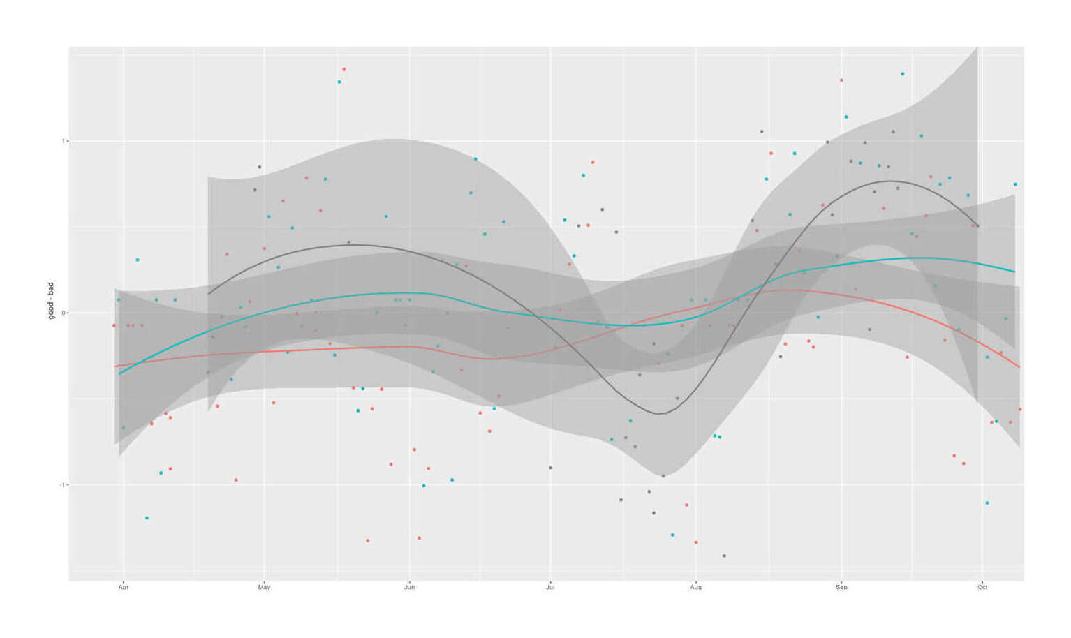
Latent sleep quality factors extracted from 9 Zeo sleep experiments and compared by ZMA supplementation status
The latent variables look sensible, with the variables loading in the expected directions. Combining the information across sleep variables sharpens the ZMA estimates in the beneficial directions (more good sleep, less bad sleep), but the graph is unconvincing and the posterior estimates are still weak, with ~77%/80% probabilities respectively of desirable effects:
## munging the MCMC matrix/lists, appears to be variables 26,27 as of 2018-01-04, blavaan version 0.2-4:
# beta[9,11,1]     -0.064641    0.042357  0.14972     0.042289   0.0548   -- 0.00045562     0.8 14466   0.035169  1.0001
posteriorGood <- s1@external$mcmcout$mcmc[1][,26][[1]]
# beta[10,11,1]     -0.11429   -0.033242 0.046418    -0.033257 0.040809   -- 0.00049508     1.2  6795    0.11383  1.0003
posteriorBad <- s1@external$mcmcout$mcmc[1][,27][[1]]
mean(posteriorGood>0)
# [1] 0.77425
mean(posteriorBad<0)
# [1] 0.802
A d = 0.04 (the factor is standardized) is a weak effect and not particularly exciting. The higher end effect-size estimates might be worth paying for but are also not especially probable (eg. d>=0.10 is only P = 14%). Ultimately, I didn’t learn much about ZMA’s effects from this experiment.
Decision
Even without a formal decision analysis, given the estimated annual cost of ~$121.34$902017, ZMA is not worth taking on the basis of this self-experiment. Should I run further experiments? For this experiment, I was troubled by the amount of data which was NA and issues with my Zeo being reliable, possibly related to older issues involving inadequate wall socket voltage (bad wiring). It would take more sampling than usual to get a meaningful amount of data1, and I still wouldn’t be able to trust the results too much because I don’t know what the problem is or how to fix or model it. So while ZMA might be worth experimenting on further, I think ZMA (or other) experiments would be pointless until I can fix my Zeo data issues.
Quickly testing by the crude approach of simply concatenating the data to itself, even doubling the data is not enough to provide high confidence, and only boosts d > 0.10 from 14% to 19%.↩︎