Diet Variance: Soylent study
Proposal to use meal-replacements to partition daily variance in mood/productivity between diet and other factors
I do not usually pay much attention to nutrition concerns. The field of nutrition has discredited itself by its allegiance to non-randomized designs despite decades of failure, and its recommendations are often harmful or not worth the cost, so for my own diet, I focus on ease of preparation, inexpensiveness, and to a lesser degree, being tasty. So there’s nothing special about it but to give an idea of what I am comparing Soylent to, I will describe typical meals.
For breakfast, I typically have 3 eggs poached or fried or as a cheese omelette, a scoop of brown rice, a scoop of a frozen vegetable (carrots, spinach, green beans), some spoons of kimchi to go with the eggs’ whites, and tea. Possibly a banana if any are left from my monthly grocery shopping, and if I have any bacon or scrapple, I will cook 2-3 slices. If not that, I might have some fresh sourdough I’ve baked myself in my oven the previous day or in my bread machine that morning using the timer (I like sourdough bread a lot, and it’s nice to wake up to the aroma of freshly-baked bread); bread recipes I use range from normal white sourdough to rye sourdough to Parmesan-onion or pesto or French peppercorn bread. If not that, I might have a big bowl of oatmeal flavored with sugar-free jam. Once in a great while, I will make pancakes with my sourdough starter or Bisquick.
For lunch, I often have a bowl of soup. I like soups and stews because they can be prepared in batches, reheat quickly, and are cheap. So I often have a crockpot of chili, spinach & rice soup, bacon & lentil soup, split pea & ham soup, beef barley soup, salmon corn chowder, carrot & coriander soup, spicy carrot soup, chunky chicken soup, chicken chowder soup, etc. If not that, then usually 2 PBJ sandwiches or grilled cheese sandwiches. Or possibly more butter bread, or BLTs if our tomatoes are in season. My fig tree produces a few figs each year, and our pear trees are abundant, so in late summer I can have those for snacks.
Dinner is a variant of lunch. Sometimes I cook fancier things like beef bourguignon or beef pot roast. Dessert might be Greek yogurt mixed with some sugar-free jam.
Time comparison of my regular food & Soylent 1.0, inclusive of total shopping, meal prep, consumption, & cleanup time:
2015-09-16: standard egg/rice/spinach/kimchi breakfast: 18m33s; bread lunch: 3m; lentil soup dinner: 17.3m; second dinner of sausage: 22m
2015-09-17: breakfast, 26m30s; grocery planning/shopping/putting-away/post-shopping-meal, 3h17m
2015-09-18: breakfast, 19m22s; dinner, 26m33s; dessert, 15m
2015-09-19: breakfast, 21m31s; cooking chili & pear picking, 1h58m; oatmeal dinner, 5m
2015-09-20: breakfast, 25m; bread, 8m30s; lunch, 19m
2015-09-21: breakfast, 44m; dinner, 27m
2015-09-22: breakfast, 38m; pear sauce, 1h19m
2015-09-23: breakfast, 30m; lunch, 20m; dinner, 25m
2015-09-24: breakfast, 24m; lunch, 30m
2015-09-25: breakfast, 18m
2015-09-26: breakfast, 21m
2015-09-27: breakfast, 28m; lunch, 10m
2015-09-28: breakfast, 18m
Soylent orders:
7 bags of 1.5; 2015-09-28 (1 bag = 1 day)
7 bags of 1.5; 2015-10-23
7 bags of 1.5; 2015-12-30
7 bags of 1.5; 2016-02-3
7 bags of 1.5; 2016-03-3
7 bags of 1.5; 2016-04-1
7 bags of 1.5; 2016-05-5
7 bags of 1.5; 2016-06-4
7 bags of 1.6; 2016-10-8
24 bottles of 2.0; 2016-10-08 (5 bottles = 1 day)
Soylent usage:
2015-09-28: 2 meals
2015-09-29: 1 meal
initial impressions: much better cold. Minor grittiness goes away after sitting overnight. Soylent Inc conveniently provides a big pitcher to make your Soylent in, narrow and tall but just short enough to fit in my refrigerator’s top shelf. Well suited to shaking and pouring. Flavor is unoffensive and has a sort of nutty/oatmeal overtone. Some stomach rumblings the first night. This stomach rumbling and flatulence is a well-known effect of Soylent and I’m afraid it hasn’t gone away for me even by 2016…
2015-09-30: 3 meals
2 Oct: 1 meal
3 Oct: 2 meals
18 Oct: 1 meal
19 Oct: 2 meals
21 Oct: 1 meal
22 Oct: 1 meal
27 Oct: 1 meal
28 Oct: 1 meal
2 Nov: 1 meal
12 Nov: 1 meal
14 Nov: 1 meal
21 Nov: 1 meal
25 Nov: 1 meal
28 Nov: 1 meal
2016
19 May: 3
22 May: 3
2 June: 3
5 June: 1
6 June: 1
7 June: 1
Overall verdict on 1.5: somewhat negative. I appreciate the shelf life of Soylent 1.5 & how I worry less about food going bad and having to plan my shopping trip, it does seem to save time in preparation & cleanup even comparing to the amortized soup time, and it’s nice knowing it’s not grossly deficient in any macronutrient; but it still costs more than my usual food per day, the constant farting took months of irregular use before it went away, I still feel hungry at the end of the day, the blandness of Soylent turns out to be oppressive. Flavoring it with cocoa powder, one of the usual suggests, didn’t solve it but made it taste more like brownie mix. Even ordinary food like some fried eggs are far more satisfying, and a day eating Soylent leaves me feeling both hungry and punished, reminded of how a highly effective punishment in prisons is to take away the regular food (wretched & unhealthy as it is) & feed inmates ‘nutraloaf’. And as a backup food, I can replace it with a big container of frozen soup. Aside from its use in self-experimentation for controlling variability/noise, I don’t see myself using Soylent for anything.
Initial notes on 2.0: the shipment is extremely heavy and I’m not a fan of it taking 5 bottles a day nor of the price. Texture-wise and flavor-wise, it tastes exactly like any soy milk with a bit of vanilla flavoring and a slightly metallic aftertaste. It is somewhat better tasting cold than room temperature. Unlike 1.5, I could imagine eating this fairly regularly.
Initial notes on 1.6: It’s rice-based, somewhat less bulky than 1.5 in powder & liquid form, and tastes similar to 2.0 but without quite the metallic aftertaste; it is definitely better cold than warm. The taste is surprisingly good - better than 2.0 and much better than 1.5. While 2.0 is just good enough that I could drink it regularly, 1.6 is good enough that I slightly enjoy it.
I also tried some banana-flavored Joylent in December 2016 in the UK. It struck me as better than 1.5 but worse than 1.6/2.0.
Notes on 1.8: after the algae allergy debacle, 1.6 was withdrawn by Rosa Labs and eventually they started selling 1.8 in early 2017. I had soured enough on 1.5 that I would be uninterested if they had returned to the oat-y 1.5-style formulation, but reviewers on /r/soylent said it was similar to 1.6, so I gave it a try, and indeed, it tastes identical as best as I can recall the flavor, making me happy.
Variance Experiment
Background
One of my hobbies is gathering data & running experiments on myself. For the most part, I can take the usual experimental approaches of measure data on relevant variables such as my usual mood/productivity MP self-rating, randomize an intervention, and regress to get the mean treatment effect.
Soylent, it occurred to me, could be useful in two ways.
Estimating Importance of Daily Diet Differences
One set of data I don’t collect is data about my diet and the food I eat: this is tedious, difficult to do right (weighing portions and calculating calories or nutritional value), cannot be automated, and I don’t want to do it unless I absolutely have to - say, because diet turns out to be a large influence on my daily energy levels and explain a lot of currently unexplained variation. I could try to estimate how big the influence is by simply collecting the data and regressing on it but that would incur a lot of work for possibly little benefit.
What if I could do something easier, to just estimate the total variance attributable to differences in food rather than nailing down the exact effect of each food? It occurred to me that this was a similar setup as with the famous twin studies of the genetic heritability of traits: since one knows how related on average identical twins, fraternal twins, siblings etc. are, one can examine the variation of sets and estimate how much all genes influence traits, without ever having to sequence a genome or identify the exact effect of a particular gene. But instead of heritability with genes, it’s ‘heritability’ for food.
In this scenario, the role of identical genomes would be played by identical meals (prepared meals like those sold to dieters, or liquid meals like the notorious Soylent & its knockoffs & Mealsquares). Days on which all 3 meals were one of the identical meals would be similar to identical twins (a genetic relatedness of 1), days with 2 of 3 meals (0.66) or 1 of 3 meals identical (0.33) would be like siblings, and days of normal food would be like unrelated (0) people from the general population. Do this for a month or two, then plug daily data on mood/energy/work into one’s favorite R library along with the meal similarity for each day (which would be possible to record as compared to my exact diet), and see if the reduction in variance is something meaningful like >10%. If it’s large, then I’ve learned I may not want to neglect recording data on my diet, since apparently day-to-day differences (I suggested this some time ago and have been looking into it in more detail since.)
Improving Statistical Power of Self-Experiments
In experiments, our statistical power or ability to detect & estimate the effects of any intervention is heavily dependent on how noisy our measurements are. It is easier to measure the effects of a diet on weight when someone is standing still & nude on a scale in a quiet doctor’s office than when they are sitting fully clothed on a roller coaster; in the former scenario, if we gain 1 kilogram, that’s easy to see against a medical scale’s inherent precision & daily weight changes of a few hundred grams, while that’s hard to see against the wild swings of scores of kilograms on a roller coaster, and we express this easiness in terms of ‘effect sizes’ which compare the absolute effect (eg. +1kg) against the noise (0.5kg or 20kg) and give the relative effect (d = 2 or d = 0.05). The more noise/variance, the more data we will require for any desired level of precision. This is the fundamental three-way tradeoff in power analysis: effect sizes vs sample sizes vs precision. A large effect size can be estimated imprecisely with a small sample size, or estimated precisely with a large sample size; or a small effect can be estimated very imprecisely with a small sample size; or…
So given this trilemma, when designing an experiment, to get the most out of it, we have a few options:
we can bite the bullet and increase the sample size; this will be expensive, sometimes impossible
we can bite the other bullet and accept imprecise estimates; this often defeats the point of running an experiment
or, we can increase the effect size, thereby either letting us decrease the sample size or getting a more precise measurement; this can be done several ways
we can directly increase the magnitude of the effect and increase the numerator of the effect size: we can increase the dose of a drug, for example, or we can exercise an additional day per week. The increase doesn’t have to be sustainable - maybe we don’t have the free time to exercise 3 times a week and we’re interested in estimating the effect of exercise twice a week, but if we exercise 3 times a week, we can finish our experiment faster and extrapolate to the smaller 2 times a week. This strategy is often not possible: an intervention may be discrete, or may already be at the optimal dose (U-shaped curves are common with drugs).
we can decrease the denominator of the effect size: in other words, reduce the noise and thereby make the same effect more visible, creating a larger effect size.
Here we again have many options. The noise in an experiment comes from many sources: we are typically measuring traits using imperfect measurements while measuring them on different days at different times in different places on different people who have different lives and genetics and all sorts of things.
We can start decreasing variance by tackling these problems: doing multiple measurements on the same equipment, at the same time of day, in the same room, using the same personnel and removing extraneous factors like clothes. If we weigh people 3 times on a scale, that will be more accurate than weighing them just once; if we weigh people 3 times a day repeatedly on multiple days, that will be even more accurate (weight can change from day to day due to factors like water retention or eating a big meal the day before); if we make sure they are nude before weighing and remove clothes, then the measurement will be better still since now different fashions, or different clothes from day to day, won’t be affecting the measurement; when doing our analysis, we can match participants up and randomize pairs of people who are as similar as possible - instead of comparing a tall black man and a short Asian girl in our study of diets (who vary a great deal in weight and height and genetics and sex), we compare two white women of the same age who are 180cm tall and are within a kilogram of each other.
Or better yet, we compare two identical twins - or better still, avoiding between-subject comparisons entirely, which are noisy for all the previously listed reasons, and switching to a within-subject experiment where we compare the same person randomized to the experiment in different time periods. Ideally, we would do any experiment by comparing each person with themselves rather than other people, although this is not always possible, like with permanent interventions.
Bad measurements and unnecessary variability can greatly reduce statistical power and require far larger samples. One noteworthy example is a large Scottish between-subject experiment into the benefits of pasteurized milk on the growth of children, which employed a large mass of ordinary children as the sample; this couldn’t be done as a within-subject design, but it was still unnecessarily noisy & sample-inefficient - had this experiment been done with the available identical twins instead of ordinary children, the increase in statistical power would have been so dramatic that they could have reduced the sample size by 95%. So, it is worth giving some thought to sources of variance and whether they can be eliminated.
Should differences in daily diet composition & amount turn out to cause a noticeable percentage of variance, then using Soylent would eliminate that variance and make the effects of interventions easier to detect.
What sort of benefit might we expect? Hypothetically, on my 1-5 daily self-ratings with a variance of ~1, if diet is a possible 20% of variance, then for a moderate effect of +0.5, it would go from an effect size of d = 0.5 / √1 = 0.5 to d = 0.5 / √(1 − 0.2) = 0.56, or for a t-test powered at 80%, saving n = 24 days (total n = 126 vs 102, respectively)1; for the (highly unlikely) scenario where diet causes 50% of variance, I would save n = 60, and so on. (For comparison, Soylent 1.6 cost me in October 2016 $48.60 for 7 days, or ~$7/day, and I estimate my regular food expenses at ~$3/day, so 102 days of Soylent would have a marginal cost of $4 a day or $306. So in the 20% variance scenario, I would in effect be paying $13 to accelerate it each day, and $5 in the 50% of variance scenario.)
Design
The outcome variable is my MP self-rating; it’s not a good outcome variable, but I am still working on creating a better productivity variable using factor analysis & SEMs, so MP will have to do for now until I can revisit the data with better methods. I have MPs going back several years, so the variance of normal eating can be estimated from that and reducing the sample size requirements.
The full blown SEM apparatus of twin study designs turn out to not be necessary here as all days are expected to have the same mean (hence, ‘pairs’ of days will have zero correlation) and I can frame the problem as a test of different variances in two ‘populations’: days with 0 Soylent meals and days with 3 Soylent meals (to maximize the contrast). This can be done as an F-test. And as a side check, a t-test for difference in means (not that I expect Soylent to increase my daily ratings, but I should check for decreases).
Randomization can be done as pairs of days to avoid temporal trends.
Power
Twin and family designs are powerful and can estimate low levels of heritability with surprisingly little data - for an additive food factor explaining 10% of variance on a continuous variable using 100% vs 50% identity (MZ vs DZ), a twin power calculator indicates that >28 pairs are necessary, so >14 pairs each, or >28 days each and >56 total, which is not too bad. Unfortunately, as I know from discussions of sex-linked variance in psychology, tests of difference in variance in general populations (as opposed to differences in means) tend to be data-hungry, presumably because twin studies benefit from pairs of twins having widely distributed means.
The power of a variance test can probably be estimated with standard ANOVA-linked power routines. However, my mood/productivity self-rating is not a continuous normal variable as such routines would assume, but a discrete variable with 3 levels, which will be less informative (so any standard power routine will underestimate the power, possibly by a lot). So a power simulation is necessary.
We can simulate realistic MP data by generating normal deviates with the same population mean/SD as my current MP dataset, rounding, and then ceiling/flooring:
mp <- read.csv("~/selfexperiment/mp.csv", colClasses=c("Date", "integer"))
sd(mp$MP, na.rm=T)
# [1] 0.6947745861
mean(mp$MP, na.rm=T)
# [1] 3.127727856
M <- round(rnorm(100, mean=3.127727856, sd=0.6947745861)); M2 <- ifelse(M>4, 4, M); M3 <- ifelse(M2<2, 2, M2)
M3
#  [1] 2 3 2 3 3 2 2 3 3 2 3 3 3 2 4 4 2 3 4 3 3 2 4 3 4 3 3 4 4 2 4 3 4 3 3 4 3 3 3 2 3 3 4 3 3 3 2 3 3 3 3 4 4 3 2 4 3 3 2 2 4 3 4 3 4 2 3 2 4 3 3 3 4 4 2 4 3 3 2 4 3 2 3 4 4 3 4 3 3 3 3 3
# [93] 4 3 2 3 3 4 2 3
sd(M3)
# [1] 0.6936945446
mean(M3)
# [1] 3.06
How to generate such deviates with particular diet-related reduction in variance, though? Not too hard:
mpGenerate <- function(n, m, s, variance) {
    M <- round(rnorm(n, mean=m, sd=sqrt((1-variance))*s))
    M2 <- ifelse(M>4, 4, M)
    M3 <- ifelse(M2<2, 2, M2)
    return(M3) }
Once that is set up, it is straightforward to pass in a set of possible reductions in variance, loop over sample sizes, simulate out a few hundred 3-meal Soylent datasets, and record the result of an F-test comparing the Soylent variance with the past non-Soylent MP variance:
library(ggplot2)
library(parallel)
library(plyr)
mpGenerate <- function(n, m, s, variance) {
    M <- round(rnorm(n, mean=m, sd=sqrt((1-variance))*s))
    M2 <- ifelse(M>4, 4, M)
    M3 <- ifelse(M2<2, 2, M2)
    return(M3) }
mpVariancePowerAnalysis <- function(heritabilities, n_additional) {

 mp <- read.csv("~/selfexperiment/mp.csv", colClasses=c("Date", "integer"))
 population_m <- mean(mp$MP, na.rm=TRUE)
 population_sd <- sd(mp$MP, na.rm=TRUE)

 iters <- 1000

 results <- ldply( # merge the identical data-frames
  mclapply(heritabilities, function(heritability) { # parallelize estimation of each possible heritability
   ## preallocate space for all the possible combinations, so we don't spend all our time
   ## merging data frames
   results <- data.frame(N=rep(NA, n_additional*iters),
      Heritability=rep(NA, n_additional*iters),
      Pvalue=rep(NA, n_additional*iters),
      Ratio=rep(NA, n_additional*iters))

   for (n in 5:n_additional) {
    for (i in 1:iters) {
      allSoylent <- mpGenerate(n, population_m, population_sd, heritability*(3/3))

      test <- var.test(mp$MP, allSoylent)

      results$N[n*i]            <- n
      results$Heritability[n*i] <- heritability
      results$Pvalue[n*i]       <- test$p.value
      results$Ratio[n*i]        <- test$estimate
      }
   }
   return(results)
 }))
 return(results)
}

power <- rbind(power, mpVariancePowerAnalysis(seq(0.1, 0.5, by=0.05), 365))
powerSummary <- aggregate(Pvalue ~ N + Heritability, function(ps) { sum(ps<=0.05)/length(ps)}, data=power)

qplot(N, Pvalue, color=as.ordered(Heritability), ylab="Power", data=powerSummary) +
 labs(color="Variance", title="Detecting variance reduction due to standardization of diet/nutrition with Soylent")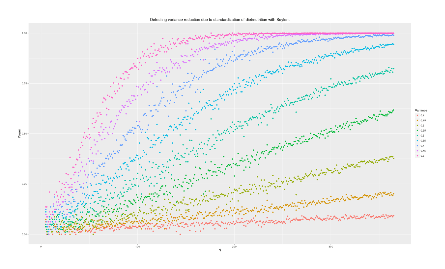
Power analysis simulation: how many additional days of Soylent-only data is necessary to detect a given reduction in variance due to removing diet/nutrition-related daily variance?
Power depends tremendously on how much variance is reduced. At an implausible 50%, a variance test is easy and requires perhaps 50 additional Soylent days; at 10%, it requires years of data. What should our prior be about effects? Some people claim that their diet affects them tremendously and eating one wrong thing (which they are not allergic to) can ruin a day; on the other hand, humans are evolved to be omnivorous and robust to disturbances in food supply (eg. the Pirahã will routinely skip a day or two of food every so often to ‘harden’ themselves) or variety of food, nor have I ever seen anything in the diet literature hinting that day to day variance might be important (researchers tending to focus on the average effects on outcome variables of particular foods like blueberries, or the effect of consistent changes in macronutrient composition, but not on how much variance/noise is due to eating more blueberries one day and less the next). I think we should expect small changes in variance, because large changes in variance attributed to diet variation must crowd out all the other possible sources like sleep, weather, blood glucose, stress and anxiety, day of the week or the lunar cycle, etc.—can all of that together really only be as large as diet shifts (as a 50% prior would claim) or only be 2x larger (as 25% claims) or only be 9x larger (as 10% claims)?
Analysis
Bayesian analysis: this is a two-group test for difference of mean & SD/variance, using interval censoring to model the discretized nature of the MP ratings. For something this simple, I could use BayesianFirstAid’s bayes.t.test(), which will estimate the variances of the two groups separately, and provides by default MCMC samples of the estimated SD for each group so one can run the test like this:
library(BayesianFirstAid)
bt <- bayes.t.test(MP ~ Soylent, data = soylent)
delta <- (bt$mcmc_samples[[1]])[,"sigma_diff"]
summary(delta); quantile(probs=c(0.025, 0.975), delta)
This doesn’t take into account the rounding of the MP into integers 1-5; if I wanted to do that, I would have to modify a two-group test to tell JAGS that the outcome variables are rounded/interval-censored:
## Demo run: read in original data, create synthetic data
mp <- read.csv("~/selfexperiment/mp.csv", colClasses=c("Date", "integer"))
mpGenerate <- function(n, m, s, variance) {
    M <- round(rnorm(n, mean=m, sd=sqrt((1-variance))*s))
    M2 <- ifelse(M>4, 4, M)
    M3 <- ifelse(M2<2, 2, M2)
    return(M3) }
population_m <- mean(mp$MP, na.rm=TRUE)
population_sd <- sd(mp$MP, na.rm=TRUE)
heritability <- 0.2
n <- 80
allSoylent <- mpGenerate(n, population_m, population_sd, heritability*(3/3))

library(runjags)
breaks <- 1:5
model1 <- "model {
    # first group:
    for (i in 1:n_1) {
    ## TODO: `dround()` is simpler than `dinterval()` but crashes for no reason I can see...
    ## posted at https://sourceforge.net/p/mcmc-jags/discussion/610037/thread/d6006dd3/
           y_1[i] ~ dinterval(true_1[i], breaks)
           true_1[i] ~ dnorm(mu_1, tau_1)
       }

    mu_1 ~ dnorm(3, pow(1, -2))
    tau_1 ~ dgamma(0.001, 0.001)
    sd_1 <- pow(tau_1, -2)

    # second group:
    for (i in 1:n_2) {
           y_2[i] ~ dinterval(true_2[i], breaks)
           true_2[i] ~ dnorm(mu_2, tau_2)
       }

    mu_2 ~ dnorm(3, pow(1, -2))
    tau_2 ~ dgamma(.001,.001)
    sd_2 <- pow(tau_2, -2)

    mu_delta <- mu_2 - mu_1

    sd_delta <- sd_2 - sd_1
    variance_ratio <- sqrt(sd_2) / sqrt(sd_1)

    }"
data <- list(breaks=breaks, y_1=mp$MP, n_1=length(mp$MP), y_2=allSoylent, n_2=length(allSoylent) )
params <- c("mu_delta", "sd_delta", "variance_ratio")
j1 <- run.jags(model=model1, monitor=params, data=data, n.chains=getOption("mc.cores"), method="rjparallel", sample=(50000/getOption("mc.cores"))); j1
Probably won’t make much of a difference.
Data
I began 2016-07-07 with 35 Soylent 1.5 bags available I had ordered over the previous months as a subscription.
8 July: 3
9 July: 0
10 July: 3
11 July: 0
12 July: 3
13 July: 0
14 July: 3
15 July: 0
16 July: 3
17 July: 0
18 July: 2
19 July: 0
9 August: 0 [long hiatus due to relatives visiting, vegetables ripening, using up my regular food before it goes bad etc.]
10 August: 3
11 August: 0
12 August: 3
13 August: 0
10 September: 3
11 September: 0
12 September: 3
13 September: 0
14 September: 3
15 September: 0
19 September: 0
20 September: 3
24 September: 0
25 September: 3
26 September: 3
27 September: 1
28 September: 3
29 September: 0
12 October: 3
13 October: 0
27 October: 0
28 October: 3
29 October: 0
30 October: 2
31 October: 3
1 November: 0
2 November: 3
3 November: 0
4 November: 0
5 November: 2
6 November: 0
7 November: 2
8 November: 3
9 November: 0
12 November: 2
13 November: 1
14 November: 1
15 November: 3
23 November: 2
2017-01-05: 0
6 January: 3
7 January: 0
8 January: 3
9 January: 0
10 January: 3
13 February: 3
14 February: 0
17 February: 0
18 February: 2
19 February: 1
23 February: 0
25 February: 3
26 February: 0
27 February: 3
28 February: 0
5 March: 0
6 March: 3
3 April: 0
4 April: 3
5 April: 0
6 April: 3
7 April: 0
8 April: 3
9 April: 0
25 April: 2
26 April: 0
27 April: 0
28 April: 3
3 May: 3
4 May: 0
19 May: 0
20 May: 1
21 May: 0
22 May: 1
23 May: 1
25 May: 0
26 May: 3
Power for the two scenarios and time savings:
↩︎power.t.test(d=0.5, power=0.80) # Two-sample t test power calculation # # n = 63.76576371 # delta = 0.5 # sd = 1 # sig.level = 0.05 # power = 0.8 # alternative = two.sided # # NOTE: n is number in *each* group power.t.test(d=0.5/sqrt(1-0.2), power=0.80) # Two-sample t test power calculation # # n = 51.21112033 # delta = 0.5590169944 # sd = 1 # sig.level = 0.05 # power = 0.8 # alternative = two.sided # NOTE: n is number in *each* group 63*2 - 51*2 # [1] 24 power.t.test(d=0.5/sqrt(1-0.5), power=0.80) # Two-sample t test power calculation # # n = 32.38447774 # delta = 0.7071067812 # sd = 1 # sig.level = 0.05 # power = 0.8 # alternative = two.sided # # NOTE: n is number in *each* group