Simulating ‘tail Collapse’ in R
N/A
A generative AI paper got a lot of press from AI-deniers by describing what it called “generative AI collapse”: a loss of modes/diversity if generative models are trained repeatedly exclusively on outputs from the previous model generation.
This is true in their highly artificial setup (which in no way resembles how generative models actually are trained & used), and also provably true in their toy model like in estimating a normal distribution: if you sample n times from 𝒩(0,1), take the empirical mean & standard deviation, and sample again, the mean will remain 0, but the SD will gradually decay to 0.
We don’t need to trust any proofs, however, as we can simply simulate this out.
In fact, it is simple enough that we can ask Claude-3 to do it in R for us!
After a little correction about what scenario exactly is being simulated & visualized, and tweaking the ggplot2 code for my preferred monochrome style, Claude-3’s coding yields:
# Set random seed for reproducibility
set.seed(42)

# Function to run a single multi-generational simulation
run_simulation <- function(n, true_mean = 0, true_sd = 100, generations = 100) {
 # Generate original sample
 sample <- rnorm(n, mean = true_mean, sd = true_sd)

 # Initialize results storage
 results <- data.frame(
 generation = 0:generations,
 mean = numeric(generations + 1),
 sd = numeric(generations + 1)
 )

 # Store original sample statistics
 results$mean[1] <- mean(sample)
 results$sd[1] <- sd(sample)

 # Run through generations
 for (i in 1:generations) {
 # Estimate parameters from the current sample
 current_mean <- mean(sample)
 current_sd <- sd(sample)

 # Generate new sample from the estimated distribution
 sample <- rnorm(n, mean = current_mean, sd = current_sd)

 # Store results
 results$mean[i + 1] <- mean(sample)
 results$sd[i + 1] <- sd(sample)
 }

 results
}

# Run simulations for different sample sizes
sample_sizes <- c(10, 100, 1000, 10000)
num_simulations <- 10000
generations <- 1000

results <- lapply(sample_sizes, function(n) {
 sim_results <- replicate(num_simulations, run_simulation(n, generations = generations),
 simplify = FALSE)

 # Average results across simulations
 avg_results <- Reduce(`+`, sim_results) / num_simulations
 avg_results$sample_size <- n
 avg_results
})

# Combine results
final_results <- do.call(rbind, results)

# Calculate percentage of original SD
final_results$sd_percentage <- final_results$sd / 100 * 100

# Print summary of results
summary_results <- final_results[final_results$generation %in% c(0, 1, 10, 50, 100), ]
print(summary_results)

# Plot the results
if (requireNamespace("ggplot2", quietly = TRUE)) {
 library(ggplot2)

 ggplot(final_results, aes(x = generation, y = sd_percentage, color = as.ordered(sample_size))) +
 scale_y_continuous(limits = c(0, 110)) +
 labs(x = "Generation", y = "Percentage of Original SD",
 title = "Standard Deviation Shrinkage Over Generations",
 color = "Sample Size") +
 geom_point(size=I(11)) +
 theme_bw(base_size = 40) + scale_color_grey()
}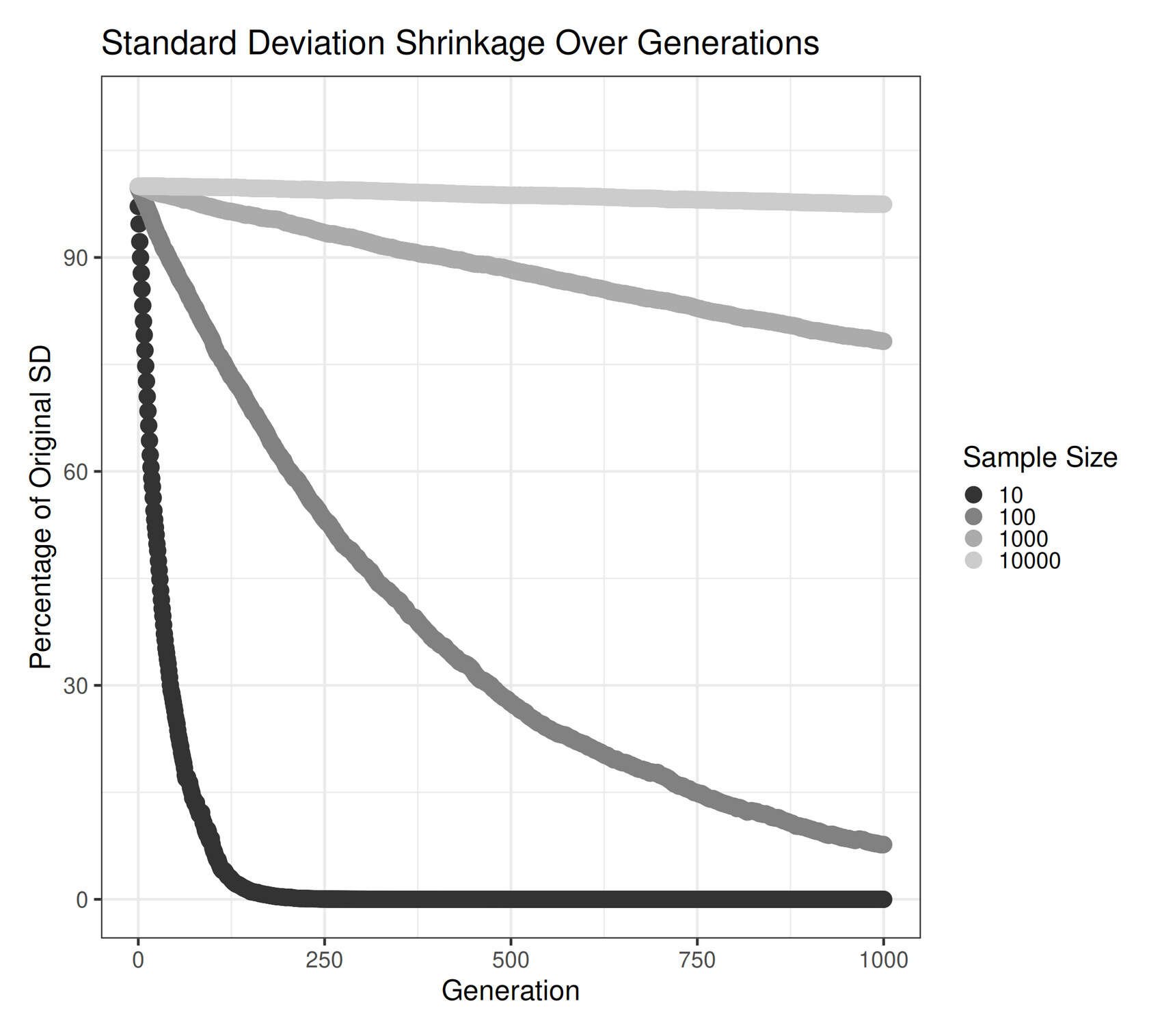
Visualizing change in standard deviation when repeatedly re-sampling.
This shows the collapse of a 𝒩(0,1) distribution over many generations of re-sampling from the empirical moments; large sample sizes can reduce the effect greatly, but it still happens.
The intuition here is that the empirical mean is an unbiased estimate of the true mean, even if it jitters around a little in a random walk; but the “uncorrected” empirical standard deviation is biased to be an underestimate—it’s easier for a sample to drop a few more extreme-than-usual points and underestimate the SD than it is to drop a few less-extreme-than-usual points & overestimate instead, so the SD tends to be an underestimate
<p>Standard implementations of the standard deviation function are not fully corrected for complex statistical reasons.</p>The R function sd implements the standard “correction” factor for defining the variance, switching n to n − 1. But it turns out that this does not fully correct it: the variance is unbiased, yes, but taking the square root of it (by Jensen’s inequality) then adds back bias!
And in fact, there is no simple fully-corrected SD: it has to be done on a distribution or case by case basis. Even the normal distribution case is more complicated than most people would want to bother with. (Such exactness would also now be incompatible with many decades of everyone else settling for the partially-corrected SD, and would be a serious problem.)
By the definition of the sampling-over-many-generations setup, this bias creates a gambler’s ruin tending to zero variance, where SD lost but not regained.
And so we observe in all scenarios a plunge (whether rapid or slow) in the standard deviation—illustrating ‘tail collapse’.