Alerts Over Time
Does Google Alerts return fewer results each year? A statistical investigation
Has Google Alerts been sending fewer results the past few years? Yes. Responding to rumors of its demise, I investigate the number of results in my personal Google Alerts notifications 2007–6201313ya, and find no overall trend of decline until I look at a transition in mid-2011 where the results fall dramatically. I speculate about the cause and implications for Alerts’s future.
While researching my Google services survival analysis essay on how long Google products survive before being killed (inspired by Reader), I came across speculation that Google Alerts, a service which runs search queries on your behalf & emails you about any new matching webpages (extremely useful for keeping abreast of topics and one of the oldest Google services), had broken badly in 201214ya. When I saw this, I remembered thinking that my own alerts did not seem to be as useful as they did, but I hadn’t been sure if this was Alerts’s fault or if my particular keywords were just less active than the past. Google’s official comments on the topic have been minimal1.
Alerts dying would be a problem for me as I have used Alerts extensively since 2007-01-28 (2347 days) with 23 current Alerts (and many more in the past) - of my 501,662 total emails, 3,815 were Alert emails - and there did not seem to be any usable alternatives2. Troublingly, Alerts’s RSS feeds were unavailable between July & September 2013.
As it happened, the survival model suggested that Alerts had a good chance of surviving a long time, and I put it from mind until I remembered that since I had used Alerts for so many years and had so many emails, I could easily check the claims empirically—did Alerts abruptly stop returning many hits? This is a straightforward question to answer: extract the subject/date/number of links from each Alerts email, stratify by unique alert, and regress over time. So I did.
Data
As part of my backup procedures, I fetch daily my Gmail emails using getmail4 into a maildir. Alerts uses an unchanging subject line like Subject: Google Alert - "Frank Herbert" -mason, so it is easy to find all its emails and separate them out.
find ~/mail/ -type f -exec grep -F -l {} 'Google Alert -' \;
# /home/gwern/mail/new/1282125775.M532208P12203Q683Rb91205f53b0fec0d.craft
# /home/gwern/mail/new/1282125789.M55800P12266Q737Rd98db4aa1e58e9ed.craft
# ...
find ~/mail/ -type f -exec grep -F -l 'Google Alert -' {} \; > alerts.txt
mkdir 2013-09-25-gwern-googlealertsemails/
mv `cat alerts.txt` 2013-09-25-gwern-googlealertsemails/
I deleted emails from a few alerts which were private; the remaining 72M of emails are available at 2013-09-25-gwern-googlealertsemails.tar.xz. Then a loop & ad hoc shell-scripting extracts the subject-line, the date, and how many instances of “http://” there are in each email:
cd 2013-09-25-gwern-googlealertsemails/

echo "Search,Date,Links" >> alerts.csv # set up the header
for EMAIL in *.craft *.elan; do

    SUBJECT="`grep -E '^Subject: Google Alert - ' $EMAIL  | sed -e 's/Subject: Google Alert - //'`"
    DATE="`grep -E '^Date: ' $EMAIL | cut -d ' ' -f 3-5 | sed -e 's/<b>..*/ /'`"
    COUNT="`grep -F --no-filename --count 'http://' $EMAIL`"

    echo $SUBJECT,$DATE,$COUNT >> alerts.csv
done
The scripting isn’t perfect and I had to delete several spurious lines before I could read it into R and format it into a clean CSV:
alerts <- read.csv("alerts.csv", quote=c(), colClasses=c("character","character","integer"))
alerts$Date <- as.Date(alerts$Date, format="%d %b %Y")
write.csv(alerts, file="2013-09-25-gwern-googlealerts.csv", row.names=FALSE)
Analysis
Descriptive
alerts <- read.csv("https://gwern.net/doc/personal/2013-09-25-gwern-googlealerts.csv",
                   colClasses=c("factor","Date","integer"))
summary(alerts)
#                      Search          Date                Links
#  wikipedia              : 255   Min.   :2007-01-28   Min.   :  0.0
#  Neon Genesis Evangelion: 247   1st Qu.:2008-12-29   1st Qu.: 10.0
#  "Gene Wolfe"           : 246   Median :2011-02-07   Median : 22.0
#  "Nick Bostrom"         : 224   Mean   :2010-10-06   Mean   : 37.9
#  modafinil              : 186   3rd Qu.:2012-06-15   3rd Qu.: 44.0
#  "Frank Herbert" -mason : 184   Max.   :2013-09-25   Max.   :563.0
#  (Other)                :2585

# So many because I have deleted many topics I am no longer interested in,
# and refined the search criteria of others
length(unique(alerts$Search))
# [1] 68

plot(Links ~ Date, data=alerts)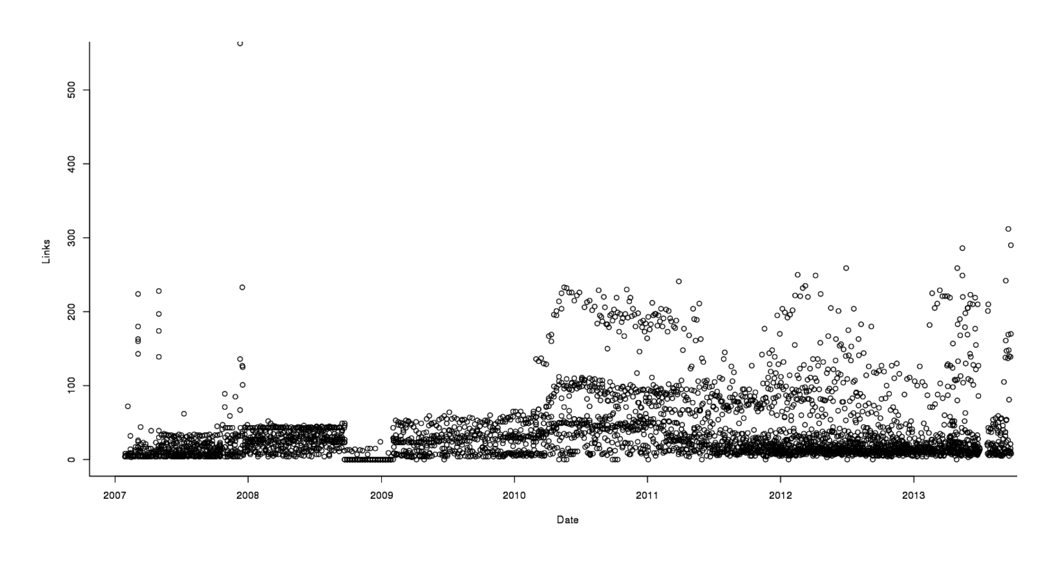
Links in each email, graphed over time
The first thing I notice is that it looks like the number of links per email is going up over time, with a spike in mid-2010. The second is that there’s quite a bit of variation from email to email - while most are around 0, some are as high as 300. The third is that there’s a weird early anomaly where emails are recorded as having 0 links; looking at those emails, they are base64 encoded, for no apparent reason, and then all subsequent emails are in more sensible HTML/text formats. An ill-fated experiment by Google? I have no idea. The highest number is 563, which isn’t very big; so despite the skew, I didn’t bother to log-transform Links.
Linear Model
The spikiness prompts me to adjust for variation in sending rate and whatnot by bucketing emails into months, and overlay a linear regression:
library(lubridate)
alerts$Date <- floor_date(alerts$Date, "month")
alerts <- aggregate(Links ~ Search + Date, alerts, "sum")

# a simple linear model agrees with *small* monthly increase, but notes that there is a tremendous
# amount of unexplained variation
lm <- lm(Links ~ Date, data=alerts); summary(lm)
# ...
# Residuals:
#    Min     1Q Median     3Q    Max
# -175.8 -110.0  -60.5   43.3  992.6
#
# Coefficients:
#              Estimate Std. Error t value Pr(>|t|)
# (Intercept) -4.13e+02   1.10e+02   -3.76  0.00018
# Date         3.73e-02   7.38e-03    5.06  4.9e-07
#
# Residual standard error: 175 on 1046 degrees of freedom
# Multiple R-squared:  0.0239,    Adjusted R-squared:  0.023
# F-statistic: 25.6 on 1 and 1046 DF,  p-value: 4.89e-07

plot(Links ~ Date, data=alerts)
abline(lm)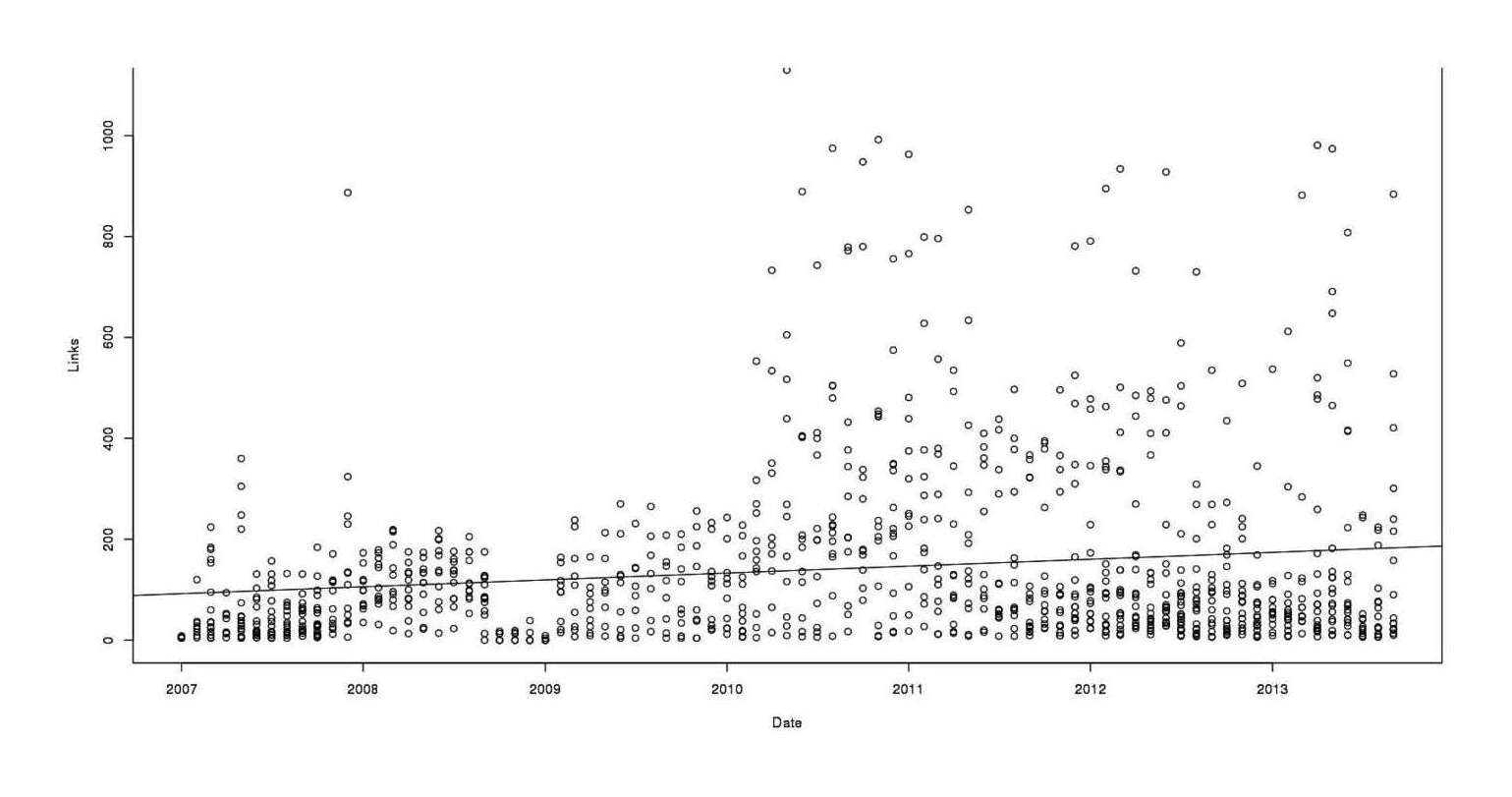
Total links in each search, by month
No big difference with the original plot: still a generic increasing trend. Here is a basic problem with this regression: does this increase reflect an increase in the number of alerts I am subscribed to, tweaks to each alert to make each return more hits (shifting from old alerts to new alerts), or an increase in links per unique alert? It is only the last claim we are interested in, but any of these or other phenomenon could produce an increase.
Per Alert
We could try treating each alert separately and doing a linear regression on them, and comparing with the linear model on all data indiscriminately:
library(ggplot2)
qplot(Date, Links, color=Search, data=alerts) +
    stat_smooth(method="lm", se=FALSE, fullrange=TRUE, size=0.2) +
    geom_abline(aes(intercept=lm$coefficients[1], slope=lm$coefficients[2], color=c()), size=1) +
    ylim(0,1130) +
    theme(legend.position = "none")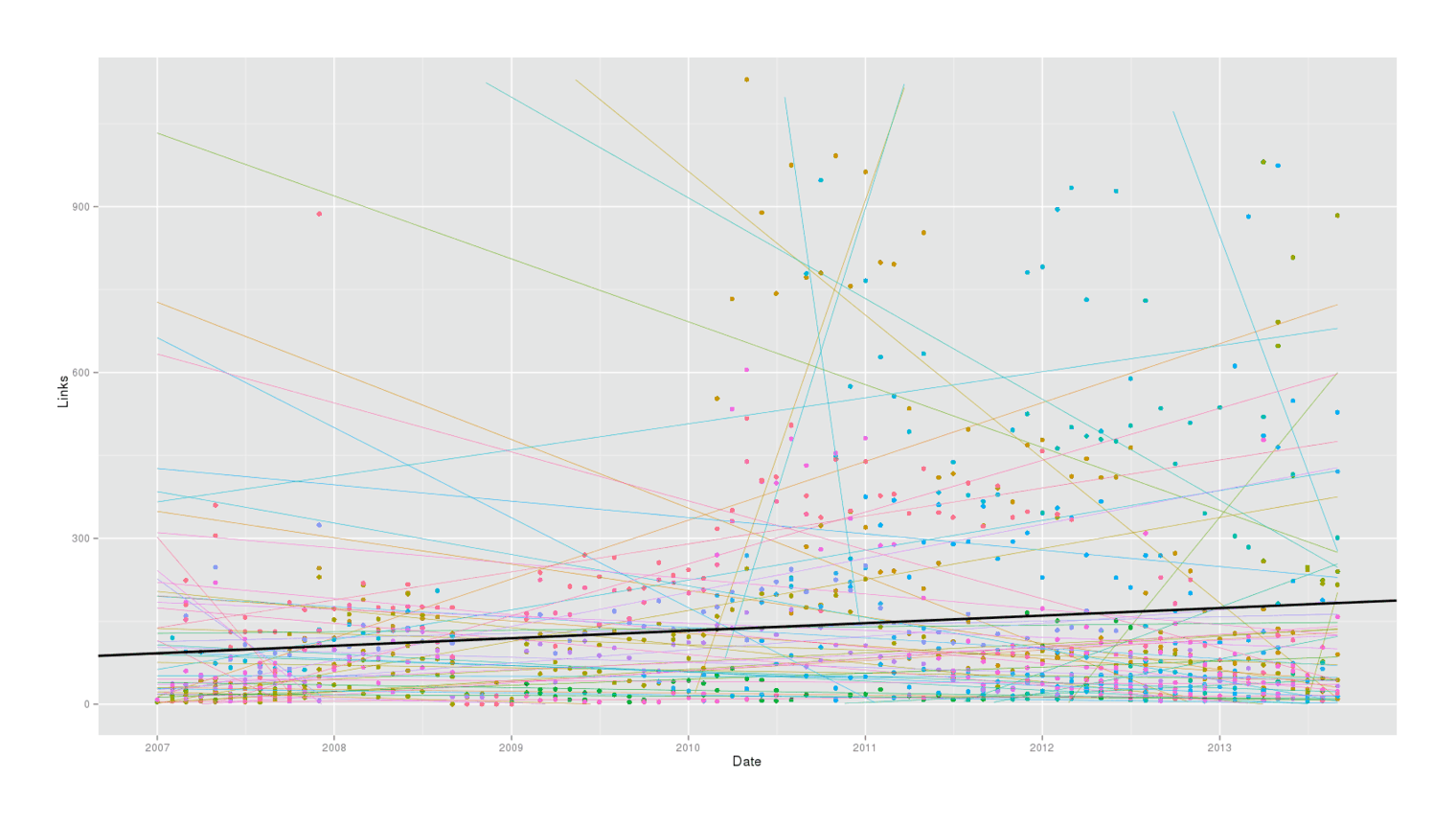
Splitting data by alert, regressing individually
The result is chaotic. Individual alerts are pointing every which way. Regressing on every alert together confounds issues, and regressing on individual alerts produces no agreement. We want some intermediate approach which respects that alerts have different behavior, but yields a meaningful overall statement.
Multi-Level Model
What we want is to look at each unique alert, estimate its increase/decrease over time, and perhaps summarize all the slopes into a single grand slope. There is a hierarchical structure to the data: the overall slope of Google influences the slope of each alert, which influences the distribution of the data points around each slope.
We can do this with a multi-level model, using lme4.
We’ll start by fitting & comparing 2 models:
only the intercept varies between each alert, but all alerts increase or decrease at the same rate
the intercept varies between each alert, and also alerts differ in their waxing or waning
library(lme4)
mlm1 <- lmer(Links ~ Date + (1|Search), alerts); mlm1
#
# Random effects:
#  Groups   Name        Variance Std.Dev.
#  Search   (Intercept) 28943    170
#  Residual             12395    111
# Number of obs: 1048, groups: Search, 68
#
# Fixed effects:
#              Estimate Std. Error t value
# (Intercept) 427.93512  139.76994    3.06
# Date         -0.01984    0.00928   -2.14
#
# Correlation of Fixed Effects:
#      (Intr)
# Date -0.988

mlm2 <- lmer(Links ~ Date + (1+Date|Search), alerts); mlm2
#
# Random effects:
#  Groups   Name        Variance Std.Dev. Corr
#  Search   (Intercept) 6.40e+06 2529.718
#           Date        2.78e-02    0.167 -0.998
#  Residual             8.36e+03   91.446
# Number of obs: 1048, groups: Search, 68
#
# Fixed effects:
#             Estimate Std. Error t value
# (Intercept) 295.5469   420.0588    0.70
# Date         -0.0090     0.0278   -0.32
#
# Correlation of Fixed Effects:
#      (Intr)
# Date -0.998

# compare the models: does model 2 buy us anything?
anova(mlm1, mlm2)
#
# mlm1: Links ~ Date + (1 | Search)
# mlm2: Links ~ Date + (1 + Date | Search)
#      Df   AIC   BIC logLik deviance Chisq Chi Df Pr(>Chisq)
# mlm1  4 13070 13089  -6531    13062
# mlm2  6 12771 12801  -6379    12759   303      2     <2e-16
Model 2 is better on both simplicity/fit criteria, so we’ll look at that closer:
coef(mlm2)
# $Search
#                                                                (Intercept)      Date
#                                                                     763.48 -0.046763
# adult iodine supplementation (IQ OR intelligence OR cognitive)      718.80 -0.043157
# AMD pacifica virtualization                                        -836.63  0.062123
# (anime OR manga) (half-Japanese OR hafu OR half-American)           956.52 -0.059438
# caloric restriction                                               -2023.10  0.153667
# "Death Note" (script OR live-action OR Parlapanides)                866.63 -0.051314
# "dual _n_-back"                                                      4212.59 -0.266879
# dual _n_-back                                                        1213.85 -0.073265
# electric sheep screensaver                                         -745.78  0.055937
# "Frank Herbert"                                                     -93.28  0.013636
# "Frank Herbert" -mason                                            10815.19 -0.676188
# freenet project                                                   -1154.14  0.087199
# "Gene Wolfe"                                                        496.01 -0.026575
# Gene Wolfe                                                         1178.36 -0.072681
# ...
# wikileaks                                                         -3080.74  0.227583
# WikiLeaks                                                          -388.34  0.031441
# wikipedia                                                         -1668.94  0.133976
# Xen                                                                 390.01 -0.017209
Date is in links per month, so when Xen has a slope of -0.02, that means that every year it falls one link.
max(abs(coef(mlm2)$Search$Date))
# [1] 0.6762
Which comes from the "Frank Herbert" -mason search, probably reflecting how relatively new the search is or the effectiveness of the filter I added to the original "Frank Herbert" search. In general, the slopes are very similar, there seem to be as many positive slopes as there are negative, and the overall summary slope is a tiny negative slope in the second model (-0.01); but most of the searches’ slopes exclude zero in the caterpillar plot:
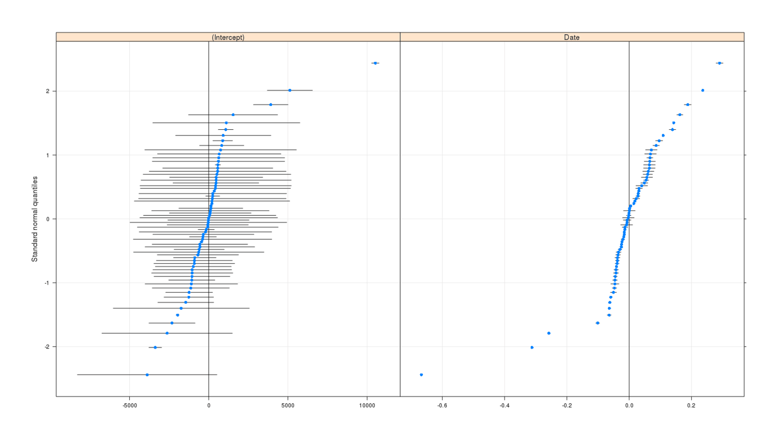
qqmath(ranef(mlm2, postVar=TRUE))
This says to me that there is no large change over time happening within each alert, as the original claims went, but there does seem to be something going on. When we plot the overall regression and the per-alert regressions, we see
fixParam <- fixef(mlm2)
ranParam <- ranef(mlm2)$Search
params   <- cbind(ranParam[1]+fixParam[1], ranParam[2]+fixParam[2])
p <- qplot(Date, Links, color=Search, data=alerts)
p +
  geom_abline(aes(intercept=`(Intercept)`, slope=Date, color=rownames(params)), data=params, size=0.2) +
  geom_abline(aes(intercept=fixef(mlm2)[1], slope=fixef(mlm2)[2], color=c()), size=1) +
  ylim(0,1130) +
  theme(legend.position = "none")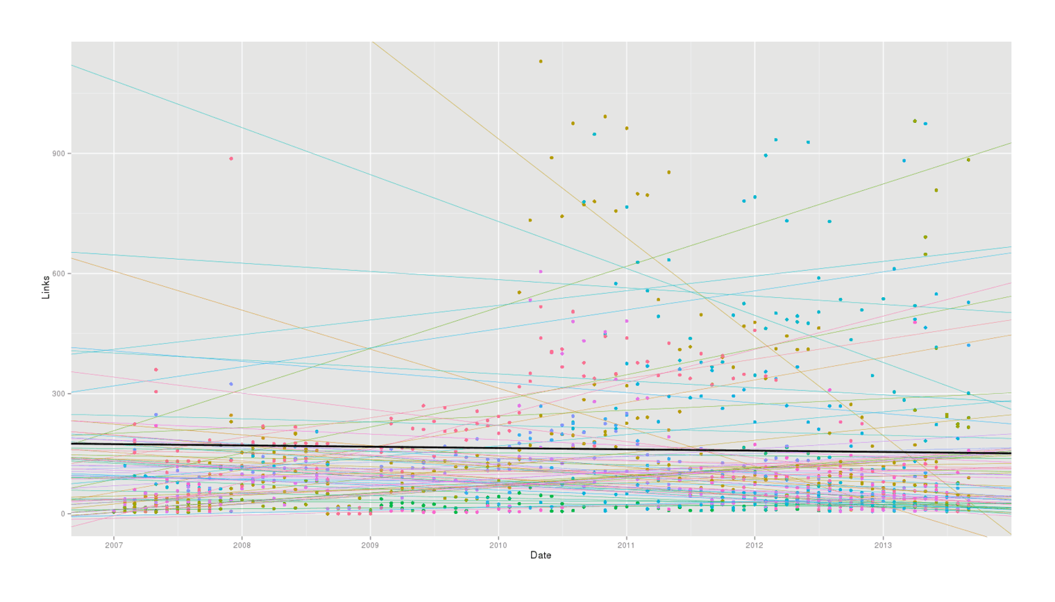
Multi-level regression, grand and individual fits
This clearly makes more sense than regressing each alert separately, as we avoid crazily steep slopes when there are just a few emails to use and their regressions get shrunk to the overall regression. We also see no evidence for any large or statistically-significant change over time for alerts in general: some alerts do increase over time but some alerts also decrease over time, and there is only a small decrease which we might blame on internal Google problems.
What about the Fall?
Having done all this, I thought I was finished until I remembered that the original bloggers didn’t complain about a steady deterioration over time, but an abrupt one starting somewhere in 201214ya. What happens when I do a binary split and compare 201016ya/201115ya to 201214ya/201313ya?
alertsRecent <- alerts[year(alerts$Date)>=2010,]
alertsRecent$Recent <- year(alertsRecent$Date) >= 2012
wilcox.test(Links ~ Recent, conf.int=TRUE, data=alertsRecent)
#
#     Wilcoxon rank sum test with continuity correction
#
# data:  Links by Recent
# W = 71113, p-value = 6.999e-10
# alternative hypothesis: true location shift is not equal to 0
# 95% confidence interval:
#  34 75
# sample estimates:
# difference in location
#                     53
I avoided a normality-based test like t.test and used instead Wilcoxon because there’s no reason to expect the number of links per month to follow a normal distribution. Regardless of the details, there’s a big difference between the two time periods: 219 vs 140 links! A fall of 36% is certainly a serious decline, and it cannot be waved away as due to my Alerts settings (I always use “All results” and never “Only the best results”) nor, as we’ll see now, a confound like the possibilities that motivated multi-level model use:
alerts$Recent <- year(alerts$Date) >= 2012
mlm3 <- lmer(Links ~ Date + Recent + (1+Date|Search), alerts); mlm3
#
# Random effects:
#  Groups   Name        Variance Std.Dev. Corr
#  Search   (Intercept) 9.22e+03 9.60e+01
#           Date        9.52e-05 9.75e-03 -0.164
#  Residual             1.18e+04 1.09e+02
# Number of obs: 1048, groups: Search, 68
#
# Fixed effects:
#              Estimate Std. Error t value
# (Intercept) -440.1540   175.3630   -2.51
# Date           0.0413     0.0121    3.42
# RecentTRUE  -102.2273    13.3224   -7.67
#
# Correlation of Fixed Effects:
#            (Intr) Date
# Date       -0.993
# RecentTRUE  0.630 -0.647
anova(mlm1, mlm2, mlm3)
# Models:
# mlm1: Links ~ Date + (1 | Search)
# mlm2: Links ~ Date + (1 + Date | Search)
# mlm3: Links ~ Date + Recent + (1 + Date | Search)
#      Df   AIC   BIC logLik deviance Chisq Chi Df Pr(>Chisq)
# mlm1  4 13070 13089  -6531    13062
# mlm2  6 12771 12801  -6379    12759   303      2     <2e-16
# mlm3  7 13015 13050  -6500    13001     0      1          1
It Was Mid-2011
A new model treating pre-2012 as different turns up with a superior fit. Can we do better? A changepoint fingers May/June 201115ya as the culprit and giving a larger difference in means (254 vs 147):
library(changepoint)
plot(cpt.meanvar(alertsRecent$Links), ylab="Links")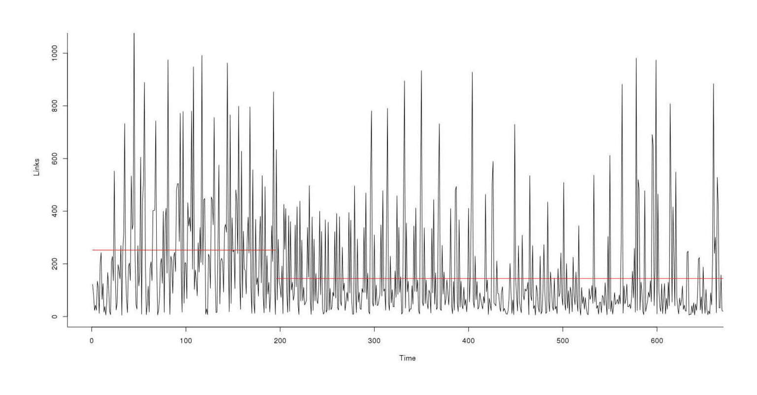
Link count 2010–201313ya, depicting a regime transition in May/June 2011
With this new changepoint, the test is more significant
alertsRecent <- alerts[year(alerts$Date)>=2010,]
alertsRecent$Recent <- alertsRecent$Date > "2011-05-01"
wilcox.test(Links ~ Recent, conf.int=TRUE, data=alertsRecent)
#
#     Wilcoxon rank sum test with continuity correction
#
# data:  Links by Recent
# W = 63480, p-value = 4.61e-12
# alternative hypothesis: true location shift is not equal to 0
# 95% confidence interval:
#   62 112
# sample estimates:
# difference in location
#                     87
And the fit improves by a large amount:
alerts$Recent <- alerts$Date > "2011-05-01"
mlm4 <- lmer(Links ~ Date + Recent + (1+Date|Search), alerts); mlm4
#
# Random effects:
#  Groups   Name        Variance Std.Dev. Corr
#  Search   (Intercept) 8.64e+03 9.30e+01
#           Date        9.28e-05 9.63e-03 -0.172
#  Residual             1.11e+04 1.05e+02
# Number of obs: 1048, groups: Search, 68
#
# Fixed effects:
#              Estimate Std. Error t value
# (Intercept) -1.11e+03   1.87e+02   -5.91
# Date         8.86e-02   1.30e-02    6.83
# RecentTRUE  -1.65e+02   1.44e+01  -11.43
#
# Correlation of Fixed Effects:
#            (Intr) Date
# Date       -0.994
# RecentTRUE  0.709 -0.725

anova(mlm1, mlm2, mlm3, mlm4)
#      Df   AIC   BIC logLik deviance Chisq Chi Df Pr(>Chisq)
# mlm1  4 13070 13089  -6531    13062
# mlm2  6 12771 12801  -6379    12759 302.7      2     <2e-16
# mlm3  7 13015 13050  -6500    13001   0.0      1          1
# mlm4  7 12948 12983  -6467    12934  66.8      0     <2e-16
Robustness
Is the fall robust against different samples of my data, using bootstrapping? The answer is yes, and the Wilcoxon test even turns out to have given us a pretty good confidence interval earlier:
library(boot)
recentEstimate <- function(dt, indices) {
  d <- dt[indices,] # allows boot to select subsample
  mlm4 <- lmer(Links ~ Date + Recent + (1+Date|Search), d)
  return(fixef(mlm4)[3])
}
bs <- boot(data=alerts, statistic=recentEstimate, R=10000, parallel="multicore", ncpus=4); bs
# ...
# Bootstrap Statistics :
#     original  bias    std. error
# t1*   -164.8   34.06       17.44

boot.ci(bs)
# ...
# Intervals :
# Level      Normal              Basic
# 95%   (-233.0, -164.7 )   (-228.2, -156.7 )
#
# Level     Percentile            BCa
# 95%   (-172.9, -101.4 )   (-211.8, -156.7 )
A confidence interval of (-159,-95) is both statistically-significant in this context and also an effect size to be reckoned with. It seems this mid-2011 fall is real. I’m surprised to find such a precise, localized, drop in my Alerts quantities. I did expect to find a decline, but I expected it to be a gradual incremental process as Google’s search algorithms gradually excluded more and more links. I didn’t expect to be able to say something like “in this month, results dropped by more than a third”.
Panda?
I don’t know of any changes announced to Google Alerts in May/June 201115ya, and the emails can’t tell us directly what happened. But I can speculate.
There is one culprit that comes to mind for what may have changed in early 201115ya which would then led to a fall in collated links (a fall which would accumulate to statistical-significance in June 201115ya): the pervasive change to webpage rankings called Google Panda. It affected many websites & searches, had teething problems, reportedly boosted social networking sites (which I generally see very few of in my own alerts), and was rolled out globally in April 201115ya - just in time to trigger a change in May/June (with continuous changes through 2011).
(We’ll probably never know the true reason: Google is notoriously uncommunicative about many of its internal technical decisions and changes.)
Conclusion
So where does this leave us?
Well, the overall linear regressions turned out to not answer the question, but they were still educational in demonstrating the considerable diversity between alerts and the trickiness of understanding what question exactly we were asking; the variability and differences between alerts reminds us to not be fooled by randomness and try to look for big effects & the big picture - if someone says their alerts seem a little down, they may have been fooled by selective memory, but when they say their alerts went from 20 links an email to 3, then we should avoid unthinking skepticism and look more carefully.
When we investigated the claim directly, we didn’t quite find the claim: there was no changepoint anywhere in 201214ya as claimed by bloggers like - they seem to have been half a year off from when the change occurred in my own alerts. What’s going on there? It’s hard to say. Google sometimes rolls out changes to users over long periods of time, so perhaps I was hit early by some changes drastically reducing links. Or perhaps it simply took time for people to become certain that there were fewer links (in which case I have given them too little credit). Or perhaps separate SEO-related changes hit their searches after mine were.
Is Alerts “broken”? Well, it’s taken a clear hit: the number of found links are down, and my own impression is that the returned links are not such gems that they make up for their gem-like rarity. And it’s certainly not good that the problem is now 2 years old without any discernible improvement.
But on closer inspection, the hit seems to have been a one-time deal, and if my Panda speculation is correct, it does not reflect any neglect or contempt by Google but simply more important factors - Search remaining high-quality will always be a higher priority than Alerts, because Search is the dog that wags the tail. My survival model may yet have the last laugh and Alerts outlast its more famous brethren.
I suppose it depends on whether you see the glass as half-full or half-empty: if half-full, then this is good news because it means that Alerts isn’t in as bad shape as it looks and may not soon be following Reader into the great Recycle Bin in the sky; if half-empty, then this is another example of how Google does not communicate with its users, makes changes unilaterally and invisibly, will degrade one service for another more profitable service, and how users are helpless in the face of its technical supremacy (who else can do as good a job of spidering the Internet for new content matching keywords?).
See Also
External Links
-
↩︎Google has refused to shed light on the decline. Today, a Google spokesperson told BuzzFeed, “we’re always working to improve our products - we’ll continue making updates to Google Alerts to make it more useful for people.” In other words, a polite non-answer.
I have seen some alternative services, Yahoo! Search Alerts, talkwalker & Mention suggested, but have not used them; the latter 2 do well in a comparison with Google Alerts.↩︎