


The past decade has seen rapid growth in research linking stable psychological characteristics (i.e., traits) to digital records of online behavior in Online Social Networks (OSNs) like Facebook and Twitter, which has implications for basic and applied behavioral sciences. Findings indicate that a broad range of psychological characteristics can be predicted from various behavioral residue online, including language used in posts on Facebook (Park et al., 2015) and Twitter (Reece et al., 2017), and which pages a person ‘likes’ on Facebook (e.g., Kosinski, Stillwell, & Graepel, 2013). The present study examined the extent to which the accounts a user follows on Twitter can be used to predict individual differences in self-reported anxiety, depression, post-traumatic stress, and anger. Followed accounts on Twitter offer distinct theoretical and practical advantages for researchers; they are potentially less subject to overt impression management and may better capture passive users. Using an approach designed to minimize overfitting and provide unbiased estimates of predictive accuracy, our results indicate that each of the four constructs can be predicted with modest accuracy (out-of-sample R’s of approximately .2). Exploratory analyses revealed that anger, but not the other constructs, was distinctly reflected in followed accounts, and there was some indication of bias in predictions for women (vs. men) but not for racial/ethnic minorities (vs. majorities). We discuss our results in light of theories linking psychological traits to behavior online, applications seeking to infer psychological characteristics from records of online behavior, and ethical issues such as algorithmic bias and users’ privacy.
Predicting Mental Health from Followed Accounts on Twitter
Stable psychological characteristics are expressed behaviorally in many domains, including online, where they often leave more or less permanent digital records in their wake. The extent to which stable individual differences in mental health are expressed online, imprinted in corresponding digital records, and ultimately recoverable from these records has wide-ranging implications for basic and applied behavioral sciences. Inferring individuals’ mental health status from online records with an appreciable degree of accuracy could accelerate advancements in clinical science, easing the burdens for researchers and participants imposed by traditional survey-based research. In time, such approaches could be developed into tools useful for clinical practice and public health. At the same time, the promise of inferring mental health from digital records of behavior is accompanied by potential threats to individuals’ privacy, as such tools could be used to infer a person’s mental health without their explicit consent. Given both the promise and risks, we need to better understand how mental health is reflected in, and recoverable from, digital records of online behavior. Our focus here is on inferring depression, anxiety, anger, and post-traumatic stress from the accounts users choose to follow on the popular online social network (OSN), Twitter.
Psychological Traits can be Inferred from Digital Records
The theory of behavioral residue holds that one by-product of the expression of traits is the accumulation of lasting residual traces of past behavior in the physical or digital spaces a person occupies. Early work demonstrated that human judges could infer psychological traits from behavioral residue in physical living and working spaces with considerable accuracy (Gosling et al., 2002). More recently, researchers have trained machine learning algorithms to do so with behavioral residue found in OSNs such as Facebook (Kosinski et al., 2013; G. Park et al., 2015; Schwartz et al., 2013). Behavioral residue in OSNs has included linguistic content (e.g., Facebook status updates; G. Park et al., 2015; Schwartz et al., 2013 and which pages a person has ‘liked’ on Facebook (Facebook-like ties; e.g., Kosinski et al., 2013), both having demonstrated considerable predictive accuracy. Indeed, the accuracy of inferences based on Facebook-like ties can even exceed that of knowledgeable human judges (Youyou et al., 2015). We focus here on using behavioral residue from Twitter, an OSN that differs from Facebook in ways relevant to basic psychological theory, public health applications, and privacy concerns.
Twitter is an OSN service and microblogging platform used by approximately 24% of US adults (as of January 2018; Pew Research Center, 2018). Users post short messages of no more than 2801 characters called “tweets” that other users can see, respond to, share (called “retweeting”), or react to (via a “like” button). Unlike Facebook, accounts are public by default, and most users choose to keep their accounts public; Twitter does not release the percentage of public accounts, but a 2009 report found that 90% of accounts were public, with a trend towards even fewer private accounts (Moore, 2009). The public nature of Twitter makes it an especially interesting setting for the present investigation for two reasons. First, its public nature eases the burden of collecting users’ data: one of several off-the-shelf Python (e.g., Tweepy; Roesslein, 2009) or R libraries (e.g., twitter; Gentry, 2015) can be used to download any of these many public accounts’ data, including their recent tweets, whom they follow, and who follows them. Thus, there is at least one fewer barrier to people outside of the Twitter company for implementing beneficial (e.g., public-health) or harmful (e.g., discriminatory) applications on Twitter than less public-facing OSNs like Facebook. Second, its public nature could affect the relative candor of behavior on Twitter, since efforts to manage others’ impressions can be stronger in more public settings (Leary & Kowalski, 1990; Paulhus & Trapnell, 2008).
Previous work has attempted to infer or predict psychological traits from behavioral residue on Twitter, focusing primarily on linguistic analyses of tweets. This growing body of work demonstrates that tweets can be used to predict a wide range of psychological characteristics, including self-reported personality traits, affective states, depression, post-traumatic stress, and the onset of suicidal ideation (Coppersmith et al., 2014; De Choudhury, Counts, et al., 2013; De Choudhury et al., 2016; De Choudhury, Gamon, et al., 2013; Dodds et al., 2011; Nadeem et al., 2016; M. Park et al., 2012; Qiu et al., 2012; Reece et al., 2017). Although the heterogeneity in how mental health is measured can make interpretation challenging, in broad terms these previous studies suggest that behavior on Twitter relates meaningfully to psychological traits. In contrast to the emphasis on linguistic analyses, there has been relatively little work using network ties on Twitter to predict psychological traits. The few attempts have looked at abstract structural characteristics of ties (e.g., tie counts or social network density; Golbeck et al., 2011; Quercia et al., 2011) rather than treating the specific accounts to which a user is tied as meaningful. We focus here on the specific accounts that users follow.
Ties or connections on Twitter are directed, meaning that users can initiate outgoing ties (called “following” on Twitter) and receive incoming ties (called “being followed” on Twitter) which are not necessarily reciprocal. In keeping with the terminology of Twitter’s Application Programming Interface (API), we refer to the group of users that a person follows as their friends and the group of users that follow a person as their followers. While both ties are likely rich in psychological meaning, we focus on friends in the present investigation for several reasons.
First, a user has nearly complete control over the accounts they follow, making friends a more direct product of the user’s own behavior. While most of a users’ followers likely reflect their own behavior and relationships, some might be unrelated (e.g., spam accounts, bots, users looking for reciprocated following, etc.), increasing the relative noise among followers (vs. friends). Second, following accounts is the primary way users’ curate their feed – what they see when they log into the app – and so their choice of friends likely reflects the information they are seeking out on Twitter. In this way, following accounts on Twitter is similar to liking pages on Facebook, a behavior which has been previously demonstrated to robustly predict psychological characteristics (Kosinski et al., 2013; Youyou et al., 2015). Third, an important practical consideration for a predictive modeling approach is that friends on Twitter often include famous brands, celebrities, politicians, or other high in-degreeaccounts, which appeal to similar interests or motivations in many users. Users are thus likely to share some friends even in moderately small samples, whereas they may have no followers in common because there aren’t parallel high out-degree accounts that appear in many users’ follower networks. Consequently, friends are far less likely to be zero-variance predictors than followers in moderately-sized, random samples.
Predicting Mental Health from Twitter-Friend Ties
Twitter-friend ties are an important next step in studying behavioral residue online for both theoretical and practical reasons. In contrast to tweets, Twitter-friend ties are not explicit signs or displays intended to be consumed by an audience of other people, and so they may be less subject to impression management goals. For this reason, Twitter-friend ties may be especially apt for predicting more evaluative psychological traits like mental health status. Likewise, people may be unaware of how much they are divulging with their selection of Twitter friends, heightening the relevant privacy concerns. For example, imagine a Twitter user who wants to present as less depressed than they truly are. They may be well aware that they should avoid writing tweets that express negative emotionality (typically the best linguistic cues for depression; see e.g., Reece et al., 2017), but they may not think to tailor their selection of friends to serve this impression management goal.
Another important advantage of Twitter-friend-based assessments is that they should work well with both active and passive users, which are distinguished in terms of the extent to which they actively engage with others (e.g., tweeting, commenting, etc.) or passively consume content (e.g., read tweets posted by their friends; Verduyn et al., 2015). Passive users tweet less often by definition, so tweet-based predictions are less suited for them. But if they are using Twitter to passively consume information, they will still follow other accounts and thus establish a set of Twitter-friend ties. Incorporating passive users may be especially advantageous for improving predictive accuracy when examining mental health such as depression and anxiety, because symptoms such as withdrawn behavior, indecision, or worry, may manifest as more passive than active twitter behavior; users who would generate insufficient data for an analysis of posted tweets may still follow a sufficient number of accounts to analyze friends.
Although the psychological meaning of Twitter friends is perhaps less immediately obvious than the psychological meaning of tweets, there are several reasons to suspect that it may be rich, and that people are therefore unknowingly disclosing sensitive information about psychological traits like anxiety, anger, depression, and post-traumatic stress through their friend networks. Individuals’ mental health could affect which accounts they choose to follow in several ways. One theory anticipating this is homophily, which holds that people like and therefore seek out others who are similar to themselves. For example, relatively depressed individuals would be anticipated to differentially follow other similarly depressed individuals or accounts. Informative to the present work, homophily has been consistently observed (offline) for individual differences in emotion (Anderson et al., 2003; Watson et al., 2000a, 2000b, 2004, 2014) and mental health status such as depression (Schaefer et al., 2011), and has recently been found in OSN friendship-ties (Youyou et al., 2017). Mental health could also affect Twitter-friend ties if selecting Twitter friends reflects strategies to regulate one’s emotions via situation selection (Gross, 2002). For example, a person who is relatively more depressed may seek out especially positive content on Twitter to upregulate positive emotions.
The reverse causal direction is also possible and Twitter friends could affect individuals’ mental health, either via emotion contagion processes – which have been observed in online social networks (Kramer et al., 2014) – or through other mechanisms. Both could affect each other complementarily, creating a person-environment transaction whereby people select themselves into networks that reinforce their existing mental health (Buss, 1984). For example, negative world views are a psychological component of depression, which may be expressed on twitter by seeking out friends that reaffirm this negative world view, which may in turn exacerbate depression symptoms. We cannot distinguish between these different possibilities in our data, but each would facilitate friend-based predictive accuracy.
The Present Study
The present study examines the extent to which psychological traits relevant to a person’s mental health and well-being can be inferred from their Twitter friends. We focused on self-reported depression, anxiety, anger, and post-traumatic stress, providing a relatively broad range of important mental health constructs. We incorporated best practices in psychometrics, open science, and machine learning. Our outcomes are measured with well-validated, psychometrically sound measures, which should enhance the predictive accuracy and explanatory utility of the results. To ensure unbiased estimates, we incorporated pre-registration and a holdout sample into our data analysis workflow, where we first performed all model training and selection in part of the data, pre-registered our final models (in a publicly-available, timestamped registration), and finally tested them on the holdout sample. In doing so, our results provide a highly rigorous test of the extent to which a broad range of mental health constructs are reflected in Twitter friend ties.
Method
Participants and Procedure
Data collection was approved by the University of Oregon Institutional Review Board (Protocol # 12082014.013) and was conducted in a manner consistent with the ethical treatment of human subjects. We collected data from the Spring of 2016 until the Fall of 2017, recruiting participants primarily from the “r/beermoney” and “r/mturk” Reddit communities, with additional participants from the University of Oregon Human Subjects Pool (UOHSP), Amazon’s Mechanical Turk (mTurk), and Twitter advertising (using promoted tweets).
Our inclusion criteria required participants to provide an existing unlocked Twitter account, currently reside in the US, speak English fluently, tweet primarily in English, and to meet minimum thresholds for being an active Twitter user. Active twitter users were defined as having a minimum of 25 tweets, 25 friends, and 25 followers. Using two-stage prescreening, we attempted to first screen participants for eligibility before they completed the main survey; participants had to affirm that they met the inclusion criteria before they proceeded with the main survey. However, since participants could erroneously state that they met the inclusion criteria, each participant was individually screened by the first author to verify that they indeed met the criteria, and to further assess whether the Twitter handle belonged to the participant whom provided it. This consisted of manually searching each Twitter account provided, ensuring it met the activity thresholds, and assessing whether the account provided was obviously fake (e.g., one participant provided Lady Gaga’s account and was subsequently excluded). When it was especially difficult to verify that the accounts provided belonged to participants, we contacted them to confirm that they indeed owned the account they provided by direct messaging our lab’s Twitter account from the account they provided.
The total number of participants recruited through each mechanism as well as the subset that were verified as meeting the inclusion criteria are shown in Table 1. As shown in Table 1, this process led to a total of Neligible = 762 accounts that we were able to verify met our inclusion criteria. Ineligible prescreen participants contained a mixture of participants who did not provide an existing Twitter account, participants who provided an account that they did not own (e.g., Lady Gaga’s account), participants whose Twitter account did not meet the activity thresholds, and participants that provided an eligible but locked account.
| Recruitment Method | NPrescreen | NEligible | NFinal |
| UOHSP | 291 | 87 | 80 |
| mTurk | 65 | 39 | 37 |
| Twitter Ads + reddit | 955 | 591 | 505 |
| 52 | 45 | 39 | |
| Total: | 1363 | 762 | 661 |
UOHSP = University of Oregon Human Subjects Pool; mTurk = Amazon’s mechanical Turk; Twitter Ads + reddit = participants recruited through promoted tweets, includes participants incidentally recruited from Reddit. Reddit = participants intentionally recruited through Reddit’s R/beermoney. NPrescreen = all participants who completed the survey before manual screening was completed. Neligible = participants who met inclusion criteria. NFinal = all participants who met inclusion criteria and we were able to get API friends data for.
In all recruitment methods, participants were able to click a link that took them to the Qualtrics survey where they provided their Twitter handles, answered some questions about their Twitter use, completed several self-report measures (described below), and finally completed basic demographics questions. At the end of the survey, participants were thanked, and compensated either with an Amazon gift card or physical check for $10 or with course credit for participants recruited through the human subjects pool.
We then downloaded each eligible participant’s full friends lists from Twitter’s API. Of the 762 eligible accounts, we were unable to get friends lists from 101 participants, one user was suspended, and the remaining 101 either deleted, locked, or changed the handle2 of their accounts in the intervening time between screening for eligibility and collecting friends lists from Twitter’s API. This resulted in the final sample for the present study of N = 661 active Twitter users. The sample consisted of 424 men and 232 women (2 did not provide gender). The majority of participants identified as White (n = 515), followed by Asian (n = 85), Black or African American (n = 44), American Indian or Alaska Native (n = 13), and Hawaiian or other Pacific Islander (n = 5). Participants could indicate more than one option, and 26 participants did. Sixty-eight participants identified as Hispanic/Latino, 590 participants identified as not Hispanic/Latino, and three provided no response. Six-hundred and thirty-five participants spoke English as their first language, 25 participants spoke English as a second language, and one participant did not indicate whether they spoke English as a first or second language.
Measures
Participants completed a series of psychometric scales, including the measures of anxiety, anger, depression, and post-traumatic stress relevant to the present study. Anxiety, anger, and depression were measured using short-forms of the Patient-Reported Outcomes Measurement Information System (PROMIS; Pilkonis et al., 2011) questionnaires. These measures asked participants to indicate the frequency of symptom occurrence on a scale ranging from 1 (never) to 5 (always). The anxiety scale consisted of eight short statements (e.g., ‘I felt fearful’), the anger scale consisted of five short statements (e.g., ‘I felt like I was ready to explode’), and the depression scale consisted of eight short statements (e.g., ‘I felt worthless’). Post-traumatic stress was measured using the well-validated 10-item Trauma Screening Questionnaire (TSQ; Brewin et al., 2002), which asks participants to indicate whether or not they have experienced 10 symptoms (‘upsetting dreams about an event’) at least twice in the past two weeks.
Planned Analyses
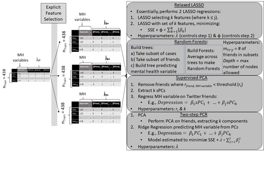
Prior to in principal acceptance, we kept ourselves blind to the data and had not conducted any analyses in any of the collected data, only manually inspecting it to ensure that it was collected correctly. This approach enabled us to write an unbiased pre-registration before running any analyses (Srivastava, 2018). After receiving in principal acceptance on September 6th 2019, we completed our registration of the approved protocol on September 10th 2019 (available at the following link: https://osf.io/5yu38). Unless otherwise noted, all analyses were conducted in R (version 3.6.1 or later; R Core Team, 2018). Figure 1 depicts our general data analysis workflow (1a), model training workflow (1b), and model testing workflow (1c). In broad strokes, our aim was to train and select a predictive model for each mental health variable that 1) maximized out-of-sample predictive accuracy, 2) guarded against over-fitting, and 3) is interpretable, providing insight into how and why mental health may be recoverable from friend relations on Twitter. To meet these aims, we partitioned our data into a training and holdout sample, performed all feature selection, data reduction, model training, and model selection on the training sample, and used the holdout sample only to assess accuracy of the final model. Our aims led us to choose four modelling approaches (detailed below) as our candidate models. We selected these four approaches based on a combination of what has worked previously with similar data in published studies (e.g., Kosinski et al., 2013) and our own feasibility studies (described later), techniques that are well-suited to Twitter friends data (e.g., algorithms that work well with sparse predictors), and potential interpretability. The specific rationale for each of the four approaches is detailed below.

Note. jall = number of unique friends in data. j3+ = number of friends with 3 or more followers in the data; j4+ = number of friends with 4 or more followers in the data; J5+ = number of friends with 5 or more followers in the data. Jselected = friends selected for testing (based on training). MH variable = mental health variable and refers to depression, anxiety, anger, and post-traumatic stress. PCA = principal components analysis. sPCs = supervised principal components. PCs = (unsupervised) principal components. Model performance during training will be determined via k-fold cross-validation (k = 10). In Figure 1c, the dashed box is unique to two-step PCR; this would not be part of the workflow for the other three approaches.

Data partitioning. As shown in Figure 1a, we first split the final sample (N = 661) into a training and holdout (testing) set using the Caret package in R (version 6.0-80; Kuhn, 2008). The training and holdout samples consist of roughly two-thirds (ntraining = 438) and one-third (nholdout = 223) of the data respectively. All feature selection, data reduction, model training, estimation, and selection were determined from the training data. The final model(s), trained and selected within the training data, were tested on the holdout sample to get an unbiased estimate of out-of-sample accuracy.
Model training. Figure 1b shows our model training workflow and approach. As seen in Figure 1b, we first conducted explicit feature selection, and then we trained and evaluated models using four different approaches (under each of the three feature selection rules). Each mental health variable was modelled separately, and so the model trained and selected for one construct (e.g., depression) could differ in every respect (approach, feature selection threshold, hyperparameters, parameters) than the model trained and selected for another construct (e.g., post-traumatic stress). All models were trained, tuned, and evaluated (within-training evaluation) using k-fold cross-validation. This splits the data into k random subsets called folds, trains the data with k-1 folds, and tests the model’s performance on the kth fold; this is repeated until each fold has been the test fold. We set k to 10, which is commonly recommended (Kosinski et al., 2016). This procedure is an efficient means for reducing overfitting during model training and selection (Yarkoni & Westfall, 2017).
Explicit feature selection. The data being used to predict mental health variables were structured as a user-friend matrix, where each row was an individual user, each column was a unique friend followed by some user(s) in the sample, and cells are filled in with 1’s or 0’s indicating whether (1) or not (0) each unique user follows each unique friend. The number of unique friends, or features (also sometimes called predictors), in the data exceeds what is computationally feasible or efficient. Moreover, accounts followed by few users are unlikely to be practically useful. At the extreme, uniquely followed accounts are effectively zero-variance predictors and therefore useless for most modeling and data reduction techniques. As such, the first step of our model training was minimal feature selection, pruning friends from the data that have few followers in our data (see Figure 1b) analogously to Kosinski and colleagues (2013) approach to Facebook likes. The optimal threshold for feature selection in this data is not yet known, so we tried three values, eliminating friends followed by fewer than 3, 4, and 5 of the participants in our data; the minimum of 3 was chosen because any lower often led to model convergence issues in the preliminary analyses (described below). The feature selection rule that showed the best training performance (see model selection section below) was used in the test data. Some modelling approachefs performed further feature selection and/or data reduction; they are described alongside the corresponding approach below.
Modelling approaches. As shown in Figure 1b, we compared four different modelling approaches: Relaxed LASSO, Random Forests, Supervised Principal Components Analysis (Supervised PCA), and two-step Principal Components Regression (PCR) with ridge regularization. Each is described in greater detail below.
Mirroring Youyou and colleagues’ (2015) approach to predicting personality from Facebook likes, we trained a model predicting each mental health variable with a variant of LASSO regression on the raw user-friend matrix, treating each unique twitter friend as a predictor variable. Classic LASSO is a penalized regression model which, like ordinary least squares (OLS), seeks to minimize the sum of squared errors and additionally seeks to minimize a function of the sum of absolute beta (regression coefficient) values (i.e., the L1 penalty, , where is a scaling parameter that determines the weight of the penalty). However, classic LASSO is known to perform poorly in contexts like these, with many noisy predictors (Meinshausen, 2007).3 Meinshausen (2007) developed relaxed LASSO to overcome this issue, by separating LASSO’s variable/feature selection function from its regularization (shrinkage) function. Essentially, it runs two LASSO regressions in sequence; the first performs variable selection, selecting k predictors (where k is ≤ total number of predictors j) based on scaling hyperparameter , and the second performs a (LASSO) regularized regression with the remaining k variables, shrinking the parameter estimates for the reduced variable set based on scaling hyperparameter ф (see Figure 2b). Relaxed LASSO, like classic LASSO, can be difficult to interpret when features are correlated, which may or may not be the case with Twitter friends in our data.
The second approach used the Random Forests algorithm on the raw user-friend matrix (see Figure 1b). Random Forests works by iteratively taking a subset of observations (or cases) and predictors, building a regression tree (i.e., a series of predictor-based decision rules to determine the value of the outcome variable) with the subset of predictors and observations, and averaging across the iterations. It is thus an ensemble method, which avoids overfitting by averaging across many models trained on a subset of participants and features. It works well with sparse predictors (Kuhn & Johnson, 2013), making it a promising candidate for Twitter friends. Like LASSO, interpretation can be difficult in the presence of correlated features. Although Relaxed LASSO and Random Forests are promising, their difficulty with correlated features could be problematic if Twitter friends are highly correlated. Our third and fourth approaches were chosen in part because they are more robust to this potential issue.
Our third approach was Supervised Principal Components Analysis (sPCA), which first conducts feature selection by eliminating features that are below some minimum (bivariate) correlation with the outcome variable, and then performs a Principal Components Regression (PCR) with the remaining feature variables; both the minimum correlation threshold and number of components to extract are traditionally determined via cross-validation (Bair et al., 2006; see Figure 1b). Interpretation tends to be relatively straightforward, even with correlated predictors, making it a promising candidate for the present aims.
Finally, mirroring Kosinski and colleagues (2013),4 we conducted a two-step PCR with ridge regularization by first conducting an unsupervised PCA on the user-friend matrix and using the resulting (orthogonal) components as predictors in a Ridge regression; we extracted the number of components that corresponded to 70% of the original variance. Ridge regression is similar to LASSO but seeks to minimize the sum of squared coefficient values (i.e., L2 penalty; ) instead; it also shrinks coefficients to be closer to zero, but tends to allow more (small) non-zero coefficients. Ridge, like LASSO, provides relatively interpretable solutions when predictors are uncorrelated, which is the case with orthogonal principal components.
Model selection. As mentioned above, all models were trained using the training data, and each model’s training performance was indexed via root mean squared error (RMSE) and the multiple correlation (R) from 10-fold cross-validation. Although machine learning approaches tend to prioritize predictive accuracy over interpretability (see Yarkoni & Westfall, 2017); we attempted to maximize both to the extent possible. As such, we selected our final model based on both (quantitative) model performance criteria (minimal RMSE, maximal multiple R) and (qualitative) interpretability. Note that in addition to RMSE/R for the best performing model, we also considered the spread of training results (e.g., we may have chosen a model that did not have the best single performance, if it had less variability in performance). We therefore selected the best fitting model that we judged to be interpretable (i.e., friends that are important in the model’s predictions made substantive sense).
Model testing. As shown in Figure 1a, we selected our candidate models based on the training data, completed an interim registration of our model selection (registered on 11/07/2019 at https://osf.io/nz7fu), and then tested the selected models’ accuracy using the (heldout) test data. After completing the interim registration, we discovered several bugs in the training analyses, and posted an addendum to the interim registration detailing them and their impact on the training results (registered on 12/19/2019 at https://osf.io/xn78h/).5 To guard against overfitting, we selected one candidate model per outcome variable. In addition to our candidate models, we also tested the out-of-sample accuracy for the non-selected models as exploratory analyses, but clearly distinguished selected from non-selected models (which can be verified in our registration). This could have included better fitting but less interpretable models, potentially providing insight into the extent to which prioritizing interpretability helps or harms out-of-sample predictive accuracy. Figure 1c shows our approach to model testing. Figure 1c highlights the independence of the model and decision making from the test data, including filtering friends (i.e., feature selection) and scoring the PCA solution (if two-step PCR is chosen). The model’s performance in the test data should thus be well-guarded against overfitting and data leakage.
Outcome-Neutral Quality Checks
We assessed the self-report and Twitter data for quality using outcome neutral criteria to better ensure that we could trust our results, especially if we were to find low predictive accuracy.
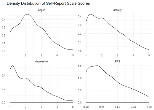
Self-report quality. To trust our predictive accuracy results we needed to ensure the quality of the self-report data. We did this in two ways. The first consisted of assessing scale reliability via split-half reliability. The second consisted of ensuring there are not floor or ceiling effects in our data by plotting distributions of scale scores. If any of the four scales had shown low reliability or evidence of a floor or ceiling effect, we would have considered that scale as having failed this quality check and consider predictive modeling with that scale less informative.
Twitter friends. Because each single friend is expected to contribute at most a small amount to predictive accuracy, our analyses rest on the presence of many (different) friends in the data. As such, we first examined the number of friends left in the data under the three feature selection thresholds we used, a minimum of 3, 4, or 5 followers in the data. We planned to not use a feature selection threshold that resulted in fewer than 100 friends unless even the least strict filter (minimum of 3 followers) did. In that event, we planned to proceed with analyses but consider this ‘minimum number of friends in the data’ quality check failed, which would be noted in the interpretation of the predictive modelling.
Preliminary Feasibility Analyses
We had conducted a series of preliminary analyses aimed at determining the feasibility of our planned approach, predicting the sentiment and emotion of user’s tweets from their Twitter friends. The scripts and data for these analyses can be found on OSF at the following link: https://osf.io/ky7u3/. We consider these to be feasibility analyses only; they do not have strong implications for our anticipated findings for at least three reasons. First, the self-report mental health variables we are seeking to predict likely have different psychometric properties than average sentiment; the former having been subject to more rigorous psychometric testing than the latter. Second, the sampling procedure here is very different than the sampling procedure we employed for the actual study. Third, the combined size of the initial samples is smaller by almost 200 participants and the replication sample is even smaller, leading to less precision. For these reasons, we believe these results speak only to the feasibility of the proposed analyses and should be interpreted primarily in this light.
Despite these differences, we conducted these analyses to explore some peculiarities of using a user-friend matrix to predict user characteristics, such as sparsity of the data. Indeed, this exercise provided valuable insights that informed our planned analyses. For example, we found that three or more followers in the data was a good lower-bound for feature selection; even relaxing this to two or more followers in the data led to model convergence issues. Likewise, we found that classic LASSO produced impossible solutions in this kind of data, whereas Relaxed LASSO did not suffer from such issues. Thus, these feasibility analyses provided a means to work out some of the issues inherent to using sparse, noisy predictors like Twitter friends.
We started by taking two samples of twitter users which were ultimately combined. The first came from a random sample of the first author’s two-step Twitter friend network (a random sample of his friends’ friends; ntwo-step-friends = 282) and the second came from a random sample of followers from two prominent political accounts (‘@BarackObama’ & ‘@realDonaldTrump’; npolitical-followers = 532). We accessed the Twitter API to download full friends lists and all available tweets for these 814 accounts. We next removed users that wouldn’t have met our inclusion criteria; users were removed if their language set to anything other than English, if they had fewer than 25 friends, and if they had fewer than 25 tweets; this resulted in a final combined sample of 484 Twitter users. We split the data into a 60-40 training-test split (ntraining = 290; ntest = 194). We then scored each of these users’ tweets for sentiment and emotion using the NRC lexicons developed for scoring sentiment and emotion in tweets (Mohammad & Kiritchenko, 2015); for the sake of space, we’ll just discuss the sentiment results here.
We predicted tweet sentiment from twitter friends’ using the approaches outlined above.6 Figure 2a contains model performance during training in these data as determined by the multiple correlation (R). The feature selection filter (i.e., the minimum number of followers in the data friends must have) is on the y-axis and multiple correlation (R) units are on the x-axis (ranging from 0 to .9 at the edge of the graph). Each dot represents a single model from training and bars represent the average across models within a given approach; the approach used is denoted by the color of the dots and bars. For example, the three (tightly clustered) purple dots at the top represent the average multiple correlation for the three Unsupervised PCA + ridge models fit with the user-friend matrix trimmed to only have friends with at least 5 followers in the data; the three models represent different values for lambda (i.e., different strengths of the L2 penalty). The accompanying purple bar is the average R across the three models.
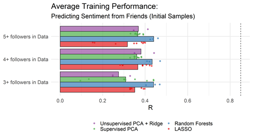
Note. Each dot represents the average multiple correlation (averaged across k-fold runs) for a model and set of hyperparameters. The bars represent the average across training runs with different hyperparameters. The dotted line at the righthand side of the graph is the split-half reliability for tweet sentiment.

As seen in Figure 2a, Random Forests with the most inclusive friends list (minimum of 3 followers in the data) had the best fitting single model (multiple R of approximately .43); Random Forests with the least inclusive friends list (minimum of 5 followers in the data) had the best average fit. We chose the former model (Random Forests with friends that have a minimum of 3 followers in the data), given that it had the best fitting single model and nearly identical average training (see Figure 2a). The out-of-sample accuracy for this model was lower than training performance, but only very slightly (R = .42). As stated previously, we additionally considered interpretability in the planned analyses, which was not part of the decision process in the feasibility analyses.
As a final step, we conducted a small replication, obtaining a small sample by sampling from follower lists of 10 popular Twitter accounts (‘@joelembiid’, ‘@katyperry’, ‘@jimmyfallon’, ‘@billgates’, ‘@oprah’, ‘@kevinheart4real’, ‘@wizkhalifa’, ‘@adele’, ‘@nba’, and ‘@nfl’); after applying the same filtering criteria as above, we had a replication sample of Nreplication = 129 unique users. We split these data into a 80-20 training-test split (nreplication_training = 103; nreplication_test = 26). The training results are displayed in Figure 2b in a graph with an identical layout to Figure 2a. As seen in Figure 2b, results looked very similar in the replication data as they did in the initial samples, with Random Forests using friends with a minimum of three followers in the data again performing best (R = .61); Random Forests using friends with a minimum of 5 followers in the data again had a slightly better average performance. We selected the former model (Random Forests, friends with 3+ followers) and again found a small decrease in predictive accuracy when applying this model to the test data (R = .48), thus confirming the relative consistency of our modelling workflow.
Results
We first assessed the outcome-neutral quality checks. For the four self-report scales, this consisted of assessing reliability (via split-half reliability) and inspecting their distributions for evidence of floor or ceiling effects. As seen in Table 2, each scale demonstrated adequate split-half reliability, had mean values close to the scale mid-points, and had the scales’ limits as minimum and maximum values. Figure 3 shows density distributions of each scale score where it is apparent that scores are somewhat positively skewed, but not to the point of suggesting floor effects that would preclude the planned analyses. The self-report scales thus demonstrated adequate reliability and did not demonstrate floor or ceiling effects, thereby passing our pre-specified outcome-neutral quality check.
| N | M | SD | Min | Max | Split-half r | |
| Depression | 658 | 2.06 | 0.94 | 1 | 5 | .95 |
| Anxiety | 658 | 2.20 | 0.94 | 1 | 5 | .94 |
| Post-Traumatic Stress | 658 | 0.33 | 0.27 | 0 | 1 | .81 |
| anger | 658 | 2.28 | 0.82 | 1 | 5 | .84 |
Split-half r corresponds to the mean split-half reliability across all possible combinations of items, calculated by the splitHalf() function from the psych library in R.
Note. PTS = post-traumatic stress.
For the followed accounts, our quality check required that more than 100 followed accounts remained after feature selection at all three selection thresholds. The total (training and holdout combined) sample of 661 participants followed 301,272 unique accounts. Filtering at three or more followers in the training data resulted in 8,422 unique followed accounts. Filtering at four or more followers in the training data resulted in 4,893 unique followed accounts. Filtering at five or more followers in the training data resulted in 3,239 unique followed accounts. Thus, each of our feature selection thresholds resulted in far more predictors than the minimally acceptable 100 from our pre-specified quality checks, and so we used each in our model training analyses.
Model Training and Selection
We trained models to predict depression, anxiety, anger, and post-traumatic stress from followed accounts. We then evaluated their cross-validated predictive accuracy and the extent to which they produced interpretable solutions (i.e., model results theoretically consistent with the construct being predicted).
Evaluating predictive accuracy. Our first major criterion for evaluating models in training was to examine their predictive accuracy, using both the correlation between predicted and observed scores (model R) and a measure of the size of models’ errors (RMSE). Rs and RMSEs were calculated using k-fold cross-validation, and corresponded to the average correlation (for R) and average difference (for RMSE) between observed and predicted scores across the 10-fold runs (in just the training data). The results of training are summarized in Figures 4 and 5. Figure 4 shows the multiple correlation for each feature selection threshold, modeling approach, and set of hyperparameters (dots) and the average across all hyperparameters (bars). Figure 5 shows the RMSE for each combination of feature selection threshold and modeling approach; the RMSE for only the best hyperparameters (per feature selection threshold and modeling approach) are shown for readability’s sake.7

Note. Each dot represents the average multiple correlation (averaged across k-fold runs) for a model and set of hyperparameters. The bars represent the average across training runs with different hyperparameters. The dotted line at the righthand side of each panel corresponds to each scale’s split-half reliability.

Note. Each dot represents the average RMSE (averaged across k-fold runs) for a model and set of hyperparameters.
As seen in Figure 4, predictive accuracy for each outcome was moderate and varied considerably across approaches and hyperparameter specifications. Using R to evaluate performance, the best-performing model for depression was random forests with accounts that have at least four followers (R = .22; RMSE = 0.94); for anxiety, supervised PCA with accounts that have at least three followers (R = .29; RMSE = 2.32); for post-traumatic stress, random forests with accounts that have at least five followers (R = .25; RMSE = 0.28); and for anger, supervised PCA with accounts that have at least five followers (R = .20; RMSE = 2.44). Using RMSE to evaluate performance, the best-performing model was random forests with at least four followers for depression (RMSE = 0.94; R = .22), anxiety (RMSE = 0.94; R = .20), and post-traumatic stress (RMSE = 0.27; R = .17), and for anger it was random forests with at least three followers (RMSE = 0.83; R = .13). Random forests thus had the lowest RMSEs across the board, and as depicted in Figure 4 it had among the highest Rs. Random forests was also robust across hyperparameter specifications, whereas some of the other modeling approaches were more sensitive to which hyperparameters were used (see Figure 4). For these reasons, we considered random forests the strongest contender by quantitative metrics.
Evaluating interpretability. Our second major criterion for model evaluation was interpretability. However, when we inspected which features were important to the different models we trained and evaluated, we saw no clear themes. As such, interpretability had basically no impact on our model selection decision (see Supplement for more details on intepretability; see Supplemental Tables S1 for followed accounts’ importance scores for selected random forests models and zero-order correlations with outcome variables).
Model Selection. Interpretability thus differed so little between approaches that it made little impact on our model selection decision, and we focused instead on the quantitative metrics reviewed above. We selected random forests for all four outcomes, because it had the lowest RMSEs and had among the highest Rs; it also tended to be robust across hyperparameter specifications. We selected a follower threshold of five for depression, anxiety, and post-traumatic stress and a threshold of four for anger based on Model Rs, RMSEs, and robustness to hyperparameter specifications. Hyperparameters for the selected models were strictly based on lowest RMSE; the best hyperparameters for all four models happened to be the same. We then wrote an interim preregistration to document our model selection decisions, saved out the best performing selected models and non-selected models, and prepared to evaluate them in the holdout data.
Model Testing
As planned in the initial pre-registered protocol, we evaluated both selected and non-selected models in the holdout data. For our central research question, estimating how well mental health can be predicted by followed accounts, we found that the selected models achieved moderate, nontrivial accuracy for all four outcomes. For depression, the correlation between predicted and observed score was R = .24, for anxiety it was R = .20, for post-traumatic stress it was R = .19, and for anger it was R = .23. Figure 6 shows these estimates.
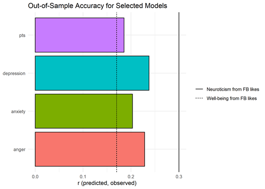
To aid in interpretation, Figure 6 also shows two relevant estimates from prior work to serve as comparative benchmarks: the predictive accuracies for well-being and neuroticism from Kosinski and colleagues’ (2013) paper predicting psychological constructs from Facebook like-ties. As seen in Figure 6, the present estimates are between these two prior estimates, suggesting that twitter friends predict mental health about as well as Facebook likes predict related constructs.
The correlations from both the selected and non-selected models are shown in Figure 7. This allows us to evaluate how effective the model-selection process was in picking the best-performing model. The selected model out-performed the eleven non-selected models for anger and post-traumatic stress, was second best for depression, and fourth best for anxiety. When one or more non-selected models outperformed the selected ones, it was by a relatively small margin, but the lowest-performing non-selected models were substantially worse than the selected ones.

Note. Asterisks indicate selected models.
To summarize, the results suggest that mental health can be predicted from followed accounts with a moderate but appreciable degree of accuracy in held-out data. Random forests generally performed well, despite the importance scores being difficult to interpret.
Exploratory Follow-up Analyses
After completing the pre-registered analyses, we completed several follow-up analyses to further explore and understand the data. In one set of analyses, we explored the specificity of prediction: were followed-account based prediction scores specific to each domain, or did they predict common variance in general psychopathology? In second set of analyses, prompted by growing public awareness of algorithmic bias in machine-learning applications, we examined the extent to which the models demonstrated predictive bias with respect to gender and race/ethnicity.
Specificity versus generality of predictive scores. Research on the structure of psychopathology has shown that disorders can be modeled with a higher-order structure, comprising broad domains like internalizing and externalizing as well as an overarching general psychopathology factor (e.g., Lahey et al., 2012; Tackett et al., 2013). In our own data the mental health scales were positively intercorrelated, with correlations in the training data ranging from .57 between post-traumatic stress and anger to .77 between anxiety and depression. We therefore wondered how much predictive performance was based on predicting specific features of each mental health construct, versus nonspecific features shared across them? To help answer this, we regressed each observed mental health variable on all four predicted scores simultaneously (within the test data). Specificity would be demonstrated by a significant slope for the matching predicted score. We observed evidence of specificity for anger (β =.24, p = .020), but effects for depression (β =.17, p = .190), anxiety (β =.11, p = .447), and post-traumatic stress (β =.04, p = .725) were not significant. This suggests that followed-account based predictions for anger captured unique features of anger. By contrast, followed-account based predictions for depression, anxiety, and post-traumatic stress may have only captured common features of a general psychopathology or internalizing factor, or specific features may have been too weak to detect in this data.
Predictive bias. Researchers and the general public are increasingly paying attention to the potential for bias in prediction algorithms (Mullainathan, 2019). Biases can be introduced into algorithms even without the knowledge or intent of their creators (such as when they are embedded in training data), and we were interested in whether the prediction models we developed might be biased. We tested for predictive bias using moderated multiple regression, a standard approach in testing and selection research (Sackett et al., 2018).
Predictive bias for gender. To test for gender bias, we regressed each observed mental health outcome variable on its corresponding predicted scores, a contrast code for the participant’s self-reported gender, and their interaction. A significant main effect of gender or an interaction between gender and predicted score would indicate that the regression lines for men and women are different, indicating the presence of bias (i.e., that men and women who the model predicts to have the same outcomes actually have different outcomes). We first tested this in the holdout data (nmen = 141; nwomen = 81) to be consistent with the out-of-sample testing results, and then also in the combined training and holdout data to increase the sample size (nmen = 424; nwomen = 232).
Figure 8 shows the relation between predicted and observed scores for men and women in the holdout data and combined data, and the results of the corresponding regression models are shown in Table 3. Starting with depression, the main effect of gender was significant in the holdout data for depression (b = 0.37, β = .40, 95% CI [.12, .68], p = .005), suggesting that women and men with the same predicted scores will differ in observed depression by .40 standard deviation units, with women being higher. However, this effect was small and indistinguishable from zero in the combined data (b = 0.03, β = .03, 95% CI [-.08, .15], p = .592).

For anxiety, the main effect of gender was significant in the holdout data (b = 0.50, β = .55, 95% CI [.27, .83], p < .001), suggesting that women and men with the same predicted scores differ by .55 standard deviation units, with women being higher. This effect was smaller and indistinguishable from zero in the combined data however (b = 0.08, β = .09, 95% CI [-.04, .21], p = .175). The interaction term was not significant in the holdout data (b = 0.22, β = .02, 95% CI [-.25, .30]. p = .876) but it was significant and moderate in size in the combined data (b = -1.28, β = -.22, 95% CI [-.34, -.10], p < .001); the latter suggests that the standardized predictive accuracy slope was weaker for women than it was for men, indicating a gender difference in how well the predicted scores can distinguish high and low anxiety, which can be seen in Figure 8.
For post-traumatic stress, the main effect of gender was significant when analyzing the holdout data alone (b = 0.15, β = .56, 95% CI [.28, .85], p < .001) and in the combined data (b = .04, β = .14, 95% CI [.02, .25], p = .027), suggesting that women and men with the same predicted scores will differ in observed post-traumatic stress, with women higher either by just over half or just over one-tenth of a standard deviation unit.
For anger, main effects of gender and the gender by prediction interactions were small and not significant in the holdout data and in the combined holdout and training data.
Going by significance, these results provide mixed evidence of gender bias in predictions of depression and anxiety, consistent evidence of bias such that women’s post-traumatic stress is systematically under-estimated, and no evidence of bias in gender bias in predictions of anger. However, the confidence intervals for the nonsignificant effects often included nontrivial amounts of bias (see Table 3), so lack of significance should not be interpreted as evidence that predictions were unbiased.
| Holdout Data | Training and Holdout Combined | |||||||||||
| b | β | 95% CI | p | b | β | 95% CI | p | |||||
| Depression | predicted | 2.16 | .17 | .04 | .31 | .013 | 4.44 | .70 | .64 | .76 | < .001 | |
| gender | 0.37 | .40 | .12 | .68 | .005 | 0.03 | .03 | -.08 | .15 | .592 | ||
| predicted X gender | 1.10 | .09 | -.18 | .36 | .525 | -0.16 | -.03 | -.14 | .09 | .652 | ||
| Anxiety | predicted | 1.09 | .11 | -.03 | .25 | .119 | 3.78 | .65 | .59 | .71 | < .001 | |
| gender | 0.50 | .55 | .27 | .83 | < .001 | 0.08 | .09 | -.04 | .21 | .175 | ||
| predicted X gender | 0.22 | .02 | -.25 | .30 | .876 | -1.28 | -.22 | -.34 | -.10 | < .001 | ||
| Post-Traumatic Stress | predicted | 0.82 | .06 | -.08 | .20 | .369 | 4.09 | .67 | .61 | .73 | < .001 | |
| gender | 0.15 | .56 | .28 | .85 | < .001 | 0.04 | .13 | .02 | .25 | .027 | ||
| predicted X gender | 1.80 | .14 | -.14 | .42 | .322 | -0.67 | -.11 | -.22 | .00 | .058 | ||
| Anger | predicted | 3.61 | .21 | .08 | .35 | .002 | 5.00 | .69 | .63 | .75 | < .001 | |
| gender | 0.11 | .13 | -.15 | .42 | .358 | -0.02 | -.02 | -.14 | .10 | .759 | ||
| predicted X gender | 2.22 | .13 | -.14 | .40 | .346 | -0.02 | .00 | -.12 | .12 | .964 | ||
Note.b refers to the unstandardized estimate; β refers to the standardized estimate; 95% CI refers to the 95% confidence interval around β. In these analyses, gender corresponds to men (nholdout = 141; ncombined = 424) vs. women (nholdout = 81; ncombined = 232); gender was contrast coded (men = -0.5; women = 0.5) so positive values for gender indicate a higher intercept for women (relative to men) and positive values for the predicted by gender interaction indicate a steeper slope for women (relative to men).
Predictive bias for race and ethnicity. We next tested for bias as a function of racial and ethnic identification. Participants indicated race (White, nholdout = 171, ncombined = 515; Asian, nholdout = 30, ncombined = 85; Black or African American, nholdout = 15, ncombined = 44; American Indian or Alaska Native, nholdout = 5, ncombined = 13; Hawaiian or other Pacific Islander, nholdout = 2, ncombined = 15; Other, nholdout = 12)8 and ethnicity (Hispanic/Latino, nholdout =24, ncombined = 68; Not Hispanic/Latino, nholdout = 198, ncombined = 590) separately. Because of small subsample sizes, we collapsed the race categories into White (nholdout = 161, ncombined = 490) vs. non-White9 (nholdout = 61, ncombined = 167), something we acknowledge raises interpretive limitations. We examined racial majorities (White) vs. minorities (non-White), ethnic majorities (not Hispanic/Latino) vs. minorities (Hispanic/Latino), and racial/ethnic majorities (White and not Hispanic/Latino; nholdout = 147, ncombined = 446) vs. minorities (either non-White or Hispanic/Latino; nholdout = 75, ncombined = 211).
The association between predicted and observed scores across race, ethnicity, and race/ethnicity are shown in Figure 9, 10, and 11 respectively; results from moderated regressions with each are shown in Tables 4, 5, and 6, respectively. There appeared to be little bias across race (see Table 4 & Figure 9), ethnicity (see Table 5 & Figure 10), or race/ethnicity (combined; see Table 6 & Figure 11) using either the holdout data (on its own) or the combined holdout and training data. However, as with gender, confidence intervals for these analyses were quite wide and generally consistent with anywhere from a moderately-sized effect in either direction to no effect (see Tables 4 – 6), highlighting that the present results are inconclusive (rather than consistent with no bias).
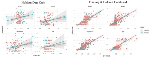


Note. Racial/Ethnic Majority = self-reported white for race and ‘Not hispanic/latino’ for ethnicity; Racial/Ethnic Minority = self-reported any other option for race or self-reported white and ‘Hispanic/Latino’ for ethnicity.
| Holdout Data | Training and Holdout Combined | |||||||||||
| b | β | 95% CI | p | b | β | 95% CI | p | |||||
| Depression | predicted | 3.06 | .24 | .09 | .40 | .002 | 4.51 | .71 | .64 | .78 | < .001 | |
| race | 0.00 | .00 | -.29 | .29 | .980 | -0.01 | -.01 | -.13 | .12 | .908 | ||
| predicted X race | 0.29 | .02 | -.28 | .33 | .880 | 0.10 | .02 | -.12 | .15 | .823 | ||
| Anxiety | predicted | 2.24 | .22 | .08 | .36 | .002 | 3.86 | .66 | .59 | .73 | < .001 | |
| race | -0.16 | -.18 | -.47 | .11 | .222 | -0.06 | -.07 | -.20 | .07 | .332 | ||
| predicted X race | 1.03 | .10 | -.18 | .38 | .469 | 0.08 | .01 | -.13 | .16 | .851 | ||
| Post-Traumatic Stress | predicted | 2.74 | .21 | .06 | .36 | .005 | 4.41 | .72 | .65 | .80 | < .001 | |
| race | 0.06 | .22 | -.07 | .51 | .144 | 0.02 | .06 | -.06 | .19 | .334 | ||
| predicted X race | 1.60 | .13 | -.17 | .43 | .410 | 0.42 | .07 | -.08 | .22 | .373 | ||
| Anger | predicted | 3.98 | .23 | .10 | .37 | .001 | 4.97 | .69 | .63 | .75 | < .001 | |
| race | -0.01 | -.01 | -.30 | .28 | .954 | -0.03 | -.03 | -.16 | .09 | .598 | ||
| predicted X race | 0.55 | .03 | -.24 | .31 | .814 | -0.10 | -.01 | -.14 | .11 | .827 | ||
Note.b refers to the unstandardized estimate; β refers to the standardized estimate; 95% CI refers to the 95% confidence interval around β. In these analyses, race was collapsed into White (nholdout = 161, ncombined = 490) vs. non-White (nholdout = 61, ncombined = 167) categories due to small sample sizes for some racial identities; race was contrast coded (White = -0.5; non-White = 0.5) so positive values for race indicate a higher intercept for non-White participants (relative to White participants) and positive values for the predicted by race interaction indicate a steeper slope for non-White participants (relative to White participants).
| Holdout Data | Training and Holdout Combined | |||||||||||
| b | β | 95% CI | p | b | β | 95% CI | p | |||||
| Depression | predicted | 3.30 | .26 | .01 | .51 | .039 | 4.66 | .74 | .64 | .84 | < .001 | |
| ethnicity | 0.08 | .08 | -.33 | .50 | .693 | 0.02 | .02 | -.16 | .20 | .841 | ||
| predicted X ethnicity | 0.72 | .06 | -.44 | .56 | .821 | 0.43 | .07 | -.13 | .27 | .502 | ||
| Anxiety | predicted | 2.67 | .27 | -.03 | .57 | .082 | 4.45 | .76 | .64 | .89 | < .001 | |
| ethnicity | 0.16 | .18 | -.26 | .62 | .422 | 0.11 | .12 | -.07 | .31 | .228 | ||
| predicted X ethnicity | 1.33 | .13 | -.47 | .73 | .663 | 1.32 | .23 | -.02 | .48 | .074 | ||
| Post-Traumatic Stress | predicted | 3.50 | .28 | .00 | .55 | .051 | 4.58 | .75 | .65 | .85 | < .001 | |
| ethnicity | 0.09 | .34 | -.10 | .77 | .126 | 0.03 | .11 | -.07 | .29 | .235 | ||
| predicted X ethnicity | 2.41 | .19 | -.36 | .74 | .499 | 0.77 | .13 | -.08 | .33 | .226 | ||
| Anger | predicted | 2.89 | .17 | -.11 | .45 | .233 | 5.43 | .75 | .65 | .86 | < .001 | |
| ethnicity | -0.13 | -.17 | -.59 | .26 | .440 | -0.01 | -.01 | -.20 | .17 | .875 | ||
| predicted X ethnicity | -2.19 | -.13 | -.69 | .43 | .651 | 0.99 | .14 | -.08 | .35 | .212 | ||
Note.b refers to the unstandardized estimate; β refers to the standardized estimate; 95% CI refers to the 95% confidence interval around β. In these analyses, ethnicity corresponds to identifying as Hispanic/Latino (nholdout = 24, ncombined = 68) or not (nholdout = 198, ncombined = 590); ethnicity was contrast coded (Not Hispanic/Latino = -0.5; Hispanic/Latino = 0.5) so positive values for ethnicity indicate a higher intercept for Hispanic/Latino participants (relative to Non-Hispanic/Latino participants) and positive values for the predicted by ethnicity interaction indicate a steeper slope for Hispanic/Latino participants (relative to Non-Hispanic/Latino participants).
| Holdout Data | Training and Holdout Combined | |||||||||||
| b | β | 95% CI | p | b | β | 95% CI | p | |||||
| Depression | predicted | 3.15 | .25 | .11 | .39 | .001 | 4.55 | .72 | .66 | .78 | < .001 | |
| race/ethnicity | 0.01 | .01 | -.26 | .29 | .924 | 0.01 | .01 | -.10 | .13 | .848 | ||
| predicted X race/ethnicity | 0.82 | .07 | -.22 | .35 | .649 | 0.29 | .05 | -.08 | .17 | .460 | ||
| Anxiety | predicted | 2.23 | .22 | .09 | .36 | .001 | 3.96 | .68 | .61 | .75 | < .001 | |
| race/ethnicity | -0.14 | -.15 | -.43 | .12 | .271 | -0.03 | -.03 | -.15 | .10 | .652 | ||
| predicted X race/ethnicity | 1.38 | .14 | -.14 | .41 | .323 | 0.46 | .08 | -.05 | .21 | .243 | ||
| Post-Traumatic Stress | predicted | 2.88 | .23 | .08 | .37 | .002 | 4.42 | .72 | .66 | .79 | < .001 | |
| race/ethnicity | 0.05 | .19 | -.08 | .47 | .173 | 0.02 | .06 | -.06 | .18 | .322 | ||
| predicted X race/ethnicity | 2.41 | .19 | -.10 | .48 | .195 | 0.57 | .09 | -.04 | .23 | .171 | ||
| Anger | predicted | 3.92 | .23 | .10 | .36 | .001 | 5.03 | .70 | .64 | .76 | < .001 | |
| race/ethnicity | -0.05 | -.06 | -.33 | .22 | .691 | -0.03 | -.03 | -.15 | .09 | .594 | ||
| predicted X race/ethnicity | 0.30 | .02 | -.25 | .28 | .897 | 0.18 | .03 | -.09 | .14 | .677 | ||
Note.b refers to the unstandardized estimate; β refers to the standardized estimate. These analyses compared racial/ethnic majority (White and not Hispanic/Latino; nholdout = 147, ncombined = 446) vs. minority participants (either non-White or Hispanic/Latino; nholdout = 75, ncombined = 211); racial/ethnic majority/minority identity was contrast coded (racial/ethnic majority = -0.5; racial/ethnic minority = 0.5) so positive values for race/ethnicity indicate a higher intercept for racial/ethnic minority participants (relative to racial/ethnic majority participants) and positive values for the predicted by race/ethnicity interaction indicate a steeper slope for racial/ethnic minority participants (relative to racial/ethnic majority participants).
Discussion
Our central aim was to understand how mental health is reflected in network connections in social media. We did so by estimating how well individual differences in mental health can be predicted from the accounts that people follow on Twitter. The results showed that it is possible to do so with moderate accuracy. We selected models in training data using 10-fold cross-validation, and then we estimated the models’ performance in new data that was kept completely separate from training, where model Rs of approximately .2 were observed. Although these models were somewhat accurate, when we examined which features were weighted as important for prediction, we did not find them to be readily interpretable with respect to prior theories or broad themes of the mental health constructs we predicted.
Mental Health and the Curation of Social Media Experiences
This study demonstrated that mental health is reflected in the accounts people follow to at least a small extent. The design and data alone cannot support strong causal inferences. One interpretation that we find plausible is that the results reflect selection processes. The list of accounts that a Twitter user follows is a product of decisions made by the user. Those decisions are the primary way that a user creates their personalized experience on the platform: when a user browses Twitter, a majority of what they see is content from the accounts they previously decided to follow. It is thus possible that different mental health symptoms affect the kind of experience people want to have on Twitter, thus impacting their followed-account list. The straightforward ways this could play-out that we discussed at the outset of this paper – e.g., face-valid information-seeking via mental health support or advocacy groups, homophily (following others who display similar mental health symptoms), or emotion regulation strategies – did not seem to be supported. Instead, the accounts with high importance scores were celebrities, sports figures, media outlets, and other people and entities from popular culture. In some rare instances, these hinted towards homophily or a similar mechanism: for example, one account with a high importance score for depression was emo-rapper Lil Peep, who was open about his struggles with depression before his untimely death. More often, however, the connections were even less obvious, and few patterns emerged across the variety of highly important predictors. Other approaches, such as qualitative interviews or experiments that manipulate different account features, may be more promising in the future for shedding light on this question.
Causality in the other direction is also plausible: perhaps following certain accounts affects users’ mental health. For example, accounts that frequently tweet depressing or angry content might elicit depression or anger in their followers in a way that endures past a single browsing session. The two causal directions are not mutually exclusive and could reflect person-situation transactional processes, whereby individual differences in mental health lead to online experiences that then reinforce the pre-existing individual differences, mirroring longitudinal findings of such reciprocal person-environment transactions in personality development (Le et al., 2014; Roberts et al., 2003). Future longitudinal studies could help elucidate whether similar processes occur with mental health and social media use.
In a set of exploratory analyses, we probed the extent to which the predicted scores were capturing specific versus general features of psychopathology. The followed-account scores that were constructed to predict anger captured variance that was unique to that construct; but for depression, anxiety, and post-traumatic stress, we did not see evidence of specificity. One possible explanation is that followed accounts primarily capture a more general psychopathology factor (Lahey et al., 2012; Tackett et al., 2013) but anger also has distinct features that are also relevant. Another possibility is that followed accounts can distinguish between internalizing and externalizing symptoms, and anger appeared to show specificity since it was the only externalizing symptom we examined. The present work cannot distinguish between these possibilities, but future work including more externalizing symptoms may be helpful in differentiating between these and other possibilities.
Relevance for Applications
What does this degree of accuracy – a correlation between predicted and observed scores of approximately .2 – mean for potential applications? First, it’s worth noting that our conclusions are limited to twitter users that meet our minimal activity thresholds (25 tweets, 25 followers, 25 followed accounts), so they may not be applicable to twitter users as a whole, including truly passive users that might follow accounts but not tweet (at all). Even among the users that do meet these thresholds, we do not believe these models are accurate enough for use in individual-level diagnostic applications, as they would provide a highly uncertain, error-prone estimate of any single individual’s mental health status. At best, a correlation of that size might be useful in applications that rely on aggregates of large amounts of data. For example, this approach could be applied to population mental health research to characterize trends in accounts from the same region or with other features in common.
A caveat is that the goal of the present study was to focus on followed accounts – not to maximize predictive power by using all available information. It may be possible to achieve greater predictive accuracy by integrating analyses of followed accounts with complementary approaches that use tweet language and other data. In addition, more advanced approaches that would be tractable in larger datasets, such as training vector embeddings for followed accounts (analogous to word2vec embeddings; Mikolov et al., 2006), could help increase accuracy and should be investigated in the future. Likewise, it may be possible to leverage findings from recent work identifying clusters or communities of high in-degree accounts (Motamedi et al., 2020, 2018) to identify important accounts or calculate aggregate community scores, as opposed to the bottom-up approaches to filtering and aggregating accounts used in this study. Future work can examine the extent to which these different modifications to our procedure maximize predictive accuracy.
Another important caveat to consider with respect to possible applications of this work is that this approach is more suited to studying more stable individual differences in mental health rather than dynamic, within-person fluctuations or responses to specific events. This was an aim that was reflected in the design of this study – for example, the wording of the mental health measures covered a broader time span than just the moment of data collection. Followed accounts are likely to be a less dynamic cue than other cues available on social media (e.g., language used in posts). This is not to say that network ties are unrelated to dynamic states entirely, and that possibility could be explored with different methods. For example, rather than focusing on whether accounts are followed or not, researchers could use engagements with accounts (such as liking or retweeting) to predict momentary reports of mental health symptomatology, or they could track users over time to measure new follows added after an event. The present work can only speak indirectly to these possibilities, but exploring approaches that dynamically link network ties to psychological states is a promising future direction for this work.
The present results, and the possibility of even higher predictive accuracy or greater temporal resolution with more sophisticated methods, raise important questions about privacy. The input to the prediction algorithm developed in this paper – a list of followed accounts – is publicly available for every Twitter user by default, and it is only hidden if a user sets their entire account to “private.” It is unlikely that users have considered how this information could be used to infer their mental health status or other sensitive topics. Indeed, even people who deliberately refrain from self-disclosing about their mental health online may be inadvertently providing information that could be the basis of algorithmic estimates, a possibility highlighted by the often less-than-straightforward accounts that the algorithms appeared to use in their predictions. With time, technological advancement, and research, these predictions might become even more accurate using similarly non-obvious cues in their predictions, though we cannot say how much more. In this way, the present findings are relevant for individuals to make informed decisions about whether and how to use social media. Likewise, they speak to broader issues of ethics, policy, and technology regulation at a systemic level (e.g., Tufekci, 2020). The possibility of a business, government, or other organization putting their considerable resources into using public social media data to construct profiles of users’ mental health may have useful applications in public health research, but it simultaneously raises concerns about how that may be misused. Our results suggest that accuracy is too low for such utopic or dystopic ends presently, but they highlight the possibilities, and the need for in-depth discussions about data, computation, privacy, and ethics.
Predictive Bias
Predictive algorithms can be biased with respect to gender, race, ethnicity, and other demographics, which can create and reinforce social inequality when those algorithms are used to conduct basic research or in applications (Mullainathan, 2019). When we probed for evidence of predictive bias for gender, we found somewhat inconclusive results. There was more of a pattern of bias in the smaller holdout dataset than in the combined data. In the holdout data, women showed higher observed levels of internalizing symptoms (depression, anxiety, and post-traumatic stress) than men with the same model-predicted scores. In the larger combined dataset, only post-traumatic stress showed this effect, and to a much smaller magnitude. Confidence bands in both datasets often ranged from no effect to moderately large effects in one or both directions. All together, we took this as suggestive but inconclusive evidence that the models may have been biased. If the pattern is not spurious, one possible reason may stem from the fact that the sample had more men than women. If men’s and women’s mental health status is associated with which accounts they follow, but the specific accounts vary systematically by gender, then overrepresentation of men in the training data could have resulted in overrepresentation of their followed accounts in the algorithm.
We found little to no evidence of bias with respect to race or ethnicity. The relative lack of bias is initially reassuring, but it should be considered alongside two caveats. First, it is possible that there is some amount of bias that we were unable to detect with the numbers of racial and ethnic minority participants in this dataset. This possibility is highlighted by the confidence bands, which (like gender) tended to range from no effect to moderately large effects. Second, it is possible that collapsing into White vs. non-White is obscuring algorithmic bias that is specific to various racial and ethnic identities. Our decision to combine minority racial and ethnic groups was based on the limitations of the available data, and it necessarily collapses across many substantively important differences.
In any future work to extend or apply the followed-accounts prediction method we present in this study, we strongly encourage researchers to attend carefully to the potential for algorithmic bias. We also hope that this work helps demonstrate how well-established psychometric methods for studying predictive bias can be integrated with modern machine learning methods.
Considering Generalizability At Two Levels of Abstraction
To what extent would the conclusions of this study apply in other settings? There are at least two ways to consider generalizability in this context. The first form of generalizability is a more abstract one, associated with the approach. Would it be possible to obtain similar predictive accuracy by applying this modeling approach to new data drawn from a different population, context, or time, developing a culturally-tuned algorithm for that new setting? We believe the results are likely to be generalizable in this sense. We used cross-validation and out-of-sample testing to safeguard against capitalizing on chance in estimates of accuracy. If the general principle holds that Twitter following decisions are associated with mental health, we expect that it would be possible to create predictive algorithms in a similar way in other settings.
A second, more specific way to think about generalizability is whether the particular prediction algorithms we trained in this study would generalize to entirely new samples from different settings. This is a much higher bar, and we are more skeptical that the models trained in this study would meet it. The fact that the models were not interpretable suggests that they may not have been picking up on theoretically central, universally relevant features of psychopathology. Instead, they might be picking up on real, but potentially fleeting, links between psychopathology and Twitter behavior. By analogy, consider differences between a self-report item like, “I frequently feel sad,” and an item like, “I frequently listen to Joy Division.” The first item would probably be endorsed by depressed people in a wide variety of contexts, populations, and historical eras. The second item, however, is deeply culturally embedded – it if is reflective of depression at all, that association would be highly specific to a particular group of people at a particular cultural moment. Even setting aside that Twitter itself is a product of a specific cultural and historical context, our inspection of the followed accounts suggests that they are not reflecting enduring features of psychopathology in a direct, face-valid sense. The associations with particular accounts were real in this data, but as cultural trends change, they may fade while new ones emerge.
Our results cannot speak to this form of generalizability directly, and it would require a new sample and different design to effectively speak to this. One possibility would be to collect several very different samples (e.g., sampled in different years), train models with each, and then evaluate cross-sample predictive accuracy. This would be a much stricter test of accuracy, but it would provide better justification for using model-derived scores in research or application. Such an approach might also be useful for distinguishing which accounts or features of accounts are predictive because of fleeting cultural factors, and which ones reflect stable and cross-contextually consistent associations with psychopathology.
Conclusion
We found that the accounts people follow on Twitter are associated with individual differences in depression, anxiety, post-traumatic stress, and anger. This raises important new theoretical questions about how mental health and social media use are intertwined. It also raises questions about what Twitter users may be revealing in their public social media data and how that could be used by researchers, governments, business, and other actors. Predictive accuracy was modest, suggesting practical limits for now. But as algorithms become more sophisticated and more personal data becomes available, more accurate predictions may become possible in the future, raising the stakes for how this approach could be used for good or for ill.
Contributions
Contributed to conception and design: CKC, SS, RR, MZ
Contributed to acquisition of data: CKC, SS, RR
Contributed to analysis and interpretation of data: CKC, SS, RR, MZ
Drafted and/or revised the article: CKC, SS, RR, MZ
Approved the submitted version for publication: CKC, SS, RR, MZ
Funding Information
National Institute of Mental Health under Grant # 1 R21 MH106879-01: SS, RR
National Science Foundation under NSF Grant # 1551817: SS, RR
Competing Interests
No competing interests were identified.
Data accessibility statement
The data for this study consists of friend lists for Twitter accounts linked to the users’ confidential self-reports of mental health symptoms. Because Twitter friend lists are public and include unique combinations, it is impossible to safely de-identify the data. Posting it in an unrestricted open repository would unavoidably expose the subjects’ confidential mental health reports in a way that is easy to link to their identity. In our consent process we obtained subjects’ permission to share their data with researchers who sign a data use agreement (agreeing to protect subjects’ confidentiality) and who obtain a valid IRB protocol from their institution. We will share the data on request with researchers who meet these qualifications. We have made analysis code and study registrations (including pre-registered Stage 1 protocol, model selection registration, and an addendum) available at https://osf.io/54qdm/ (also referenced in the author note; links to specific elements are provided throughout the text).
Footnotes
Prior to November 2017, tweets were limited to 140 characters.
Our workflow consisted of looking up users in Twitter’s API based on the handle they provided using application-only authentication.
We confirmed that classic LASSO is a poor fit for this kind of data; some models fit with classic LASSO during the preliminary analyses (described below) produced predicted values outside of the bounds of the observed data (indicated by RMSE values in the millions; see LASSO section of ‘predictive_modelling_both_samples.html’ at the projects’ osf site: https://osf.io/ky7u3/). Relaxed LASSO did not suffer from such issues.
One major difference between Kosinski and colleagues’ (2013) and our approach is that we used PCA instead of singular value decomposition (SVD). PCA is special case of SVD where the data matrix is first centered; because of this centering, it tends to be less computationally efficient but more interpretable. Our feasibility analyses (described below) indicate that PCAs are indeed feasible in data similar to the present data.
This addendum refers to an output file that has been removed from OSF out of an abundance of caution for participants’ privacy, but is identical to the output file in the main project repository except that exact PCA-loadings were removed and summarized textually instead (available here: https://osf.io/axgrj/)
We also used classic LASSO and found that it produced impossible predictions (RMSEs and MAEs in the millions); those can be found in the script and output for the initial samples (“predictive_modelling_both_samples.html”) but are not discussed here.
Under certain hyperparameters, relaxed LASSO resulted in RMSEs in the hundreds, rendering plots of RMSEs from all models difficult to read.
Participants could select more than one option, so these cell n’s don’t sum to the total sample sizes.
Non-White includes multiracial participants who indicated White as one of multiple racial identities.

