Written by Ethan Smith
Table of Contents
Intro
To start off, the title is a slight misnomer. Canonically, diffusion is the portion where we destroy the data into noise through random processes, and then we learn the reverse process. That doesn’t happen here.
But I kept the name because I think most people think of the generative portion when hearing the word diffusion, and there are some inspirations taken from it.
The aspect of diffusion we are trying to recover here is the ability to to synthesize images by developing low frequency components first and moving on to higher frequencies.
In short, the philosophy here is that the diffusion model generative process in the data/pixel domain is similar to sequence modeling in the frequency domain.
Kinda analogous to the common wisdom that convolution in the time domain is multiplication in the frequency domain
What I want to see here is if we can create an autoregressive transformer model that can build an image by sequentially generating its frequency components.
Potential Pros
The pros are that we can now get a loss from the entire generation process simultaneously. Normally when training diffusion models, you’ll sample a random timestep, get a prediction, and take the loss for that timestep.
Because of the parallelizability of the training of causal transformer models, we can compute the loss for the entire trajectory at once.
Granted, a single frequency coefficient is not really the same as a prediction of the entire image/noise.
Secondly, I think there’s an advantage over autoregressive methods that generate images like DALLE-1, PARTI, Cogview, and some others.
To me it always felt really strange that you would just generate all the pixels or latent tokens of an image raster scan style i.e. starting from the top left corner and going across each row.
Why should the top row of pixels have the least context and the bottom right pixel of the image have the most context?
It seems totally arbitrary, why not start from the center and spiral outward or zigzag across the image similar to how jpeg compression does it?
I mean it works because if you throw an autoregressive transformer at anything with enough data and compute it works, but I feel like it doesn’t properly leverage the nature of the data its working with.
Here by generating frequencies, we cover the entire image from the very start, and every additional frequency gets the context of the past blurrier version of the image essentially, starting off with low global certainty of the image content and gaining confidence in each step.
Potential Cons
The cons are that this method now means generation requires a fixed amount of forward passes.
Unless you’re willing to truncate the higher frequencies.
Also, with this setup, we have as many coefficients to predict as there are pixels in an image, across all channels as well, which can end up in really long sequences.
Nonetheless, it seemed like a fun thing to try!
Background
Feel free to skip this part if you’re familiar with Fourier operations, but also put in some nice visualizations of what happens in different regions with the 2D case that were somewhat new to me.
Frequencies of Data and the Fourier Transform
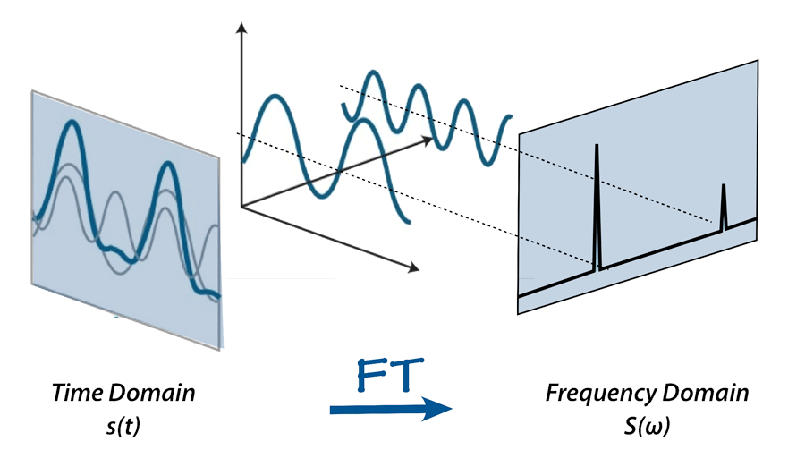
This will be a quick recap. If you’d like to learn more about frequency representations, the link in the caption of the image below gives a good overview.
When working with data like audio or images, we have the ability to extract frequency representations of our samples using the Fourier transform
A signal can be decomposed into coefficients denoting the magnitudes of sin and cosine waves of certain frequencies that compose it.
In the above example the signal is largely made up of the slower wave and in smaller part of the faster wave. On the left you can also see how by summing the waves, after multiplying them by their coefficients, we can recover the signal.
In practice also, we’ll use the complex-valued Fourier transform, which gives outputs complex numbers. The absolute value of the complex number denotes the magnitude of a given wave while the angle denotes the wave’s phase
This answer on StackExchange gives a nice visual about the role of phase and magnitude information when reconstructing a signal by showing what happens when each is dropped out. Needless to say, we’ll need both.
When working with images, we can think of the waves as the change in pixel intensity (0-255, normalized 0-1 for our case) as we move across a direction in the image.
Here’s a picture of a cute dog.
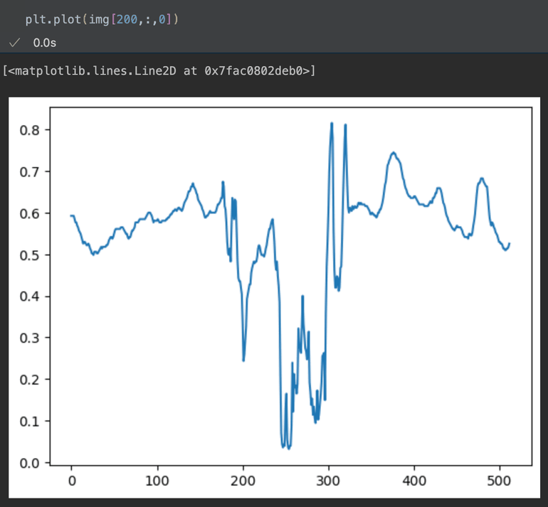
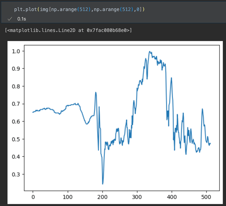
Now here’s our dog but as the red channel from the 200th row of pixels from the top plotted with their x-position in the image on the x-axis, and their intensity on the y-axis.
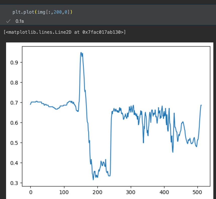
We can also do this for columns of pixels in the image
To capture the full image signal as waves, we have to consider all directions in which these waves can occur, so not just horizontal and vertical slices- we’ll also have diagonals of all angles going across the image.
This is rather hard to do via indexing a numpy array, so i’ll just show how we can extract the 45 degree diagonal across the image
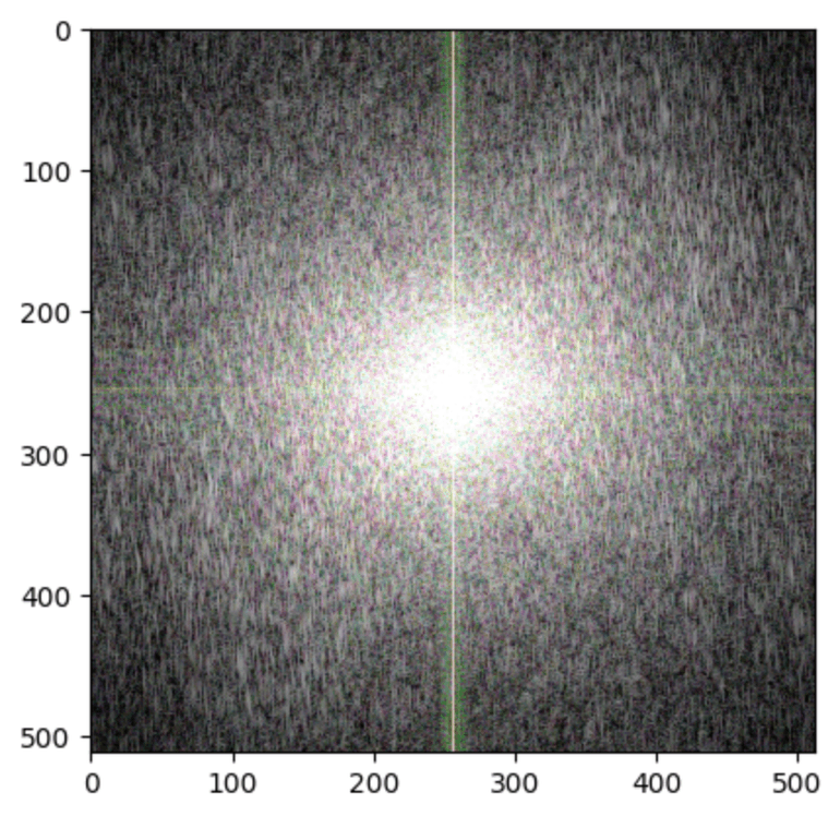
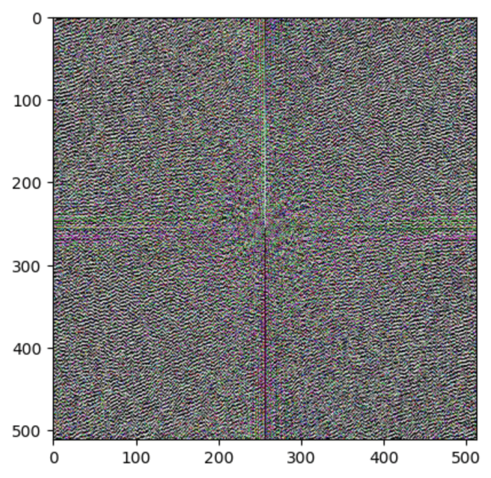
Anyway, because of this nuance, we now have to use the specialized 2D Fourier Transform. Here’s our same dog as a Great Ball Of Light after the transform.
Magnitude
Phase
Also note, because the Fourier coefficients of magnitude can range to very large and small values, I took the logarithm for better visibility.
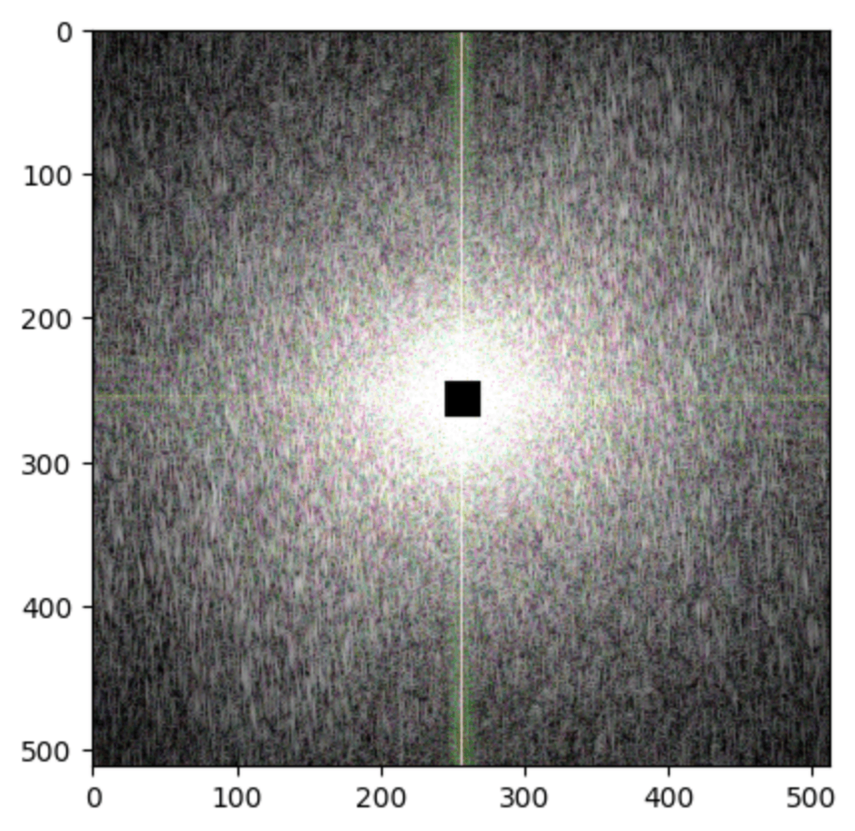
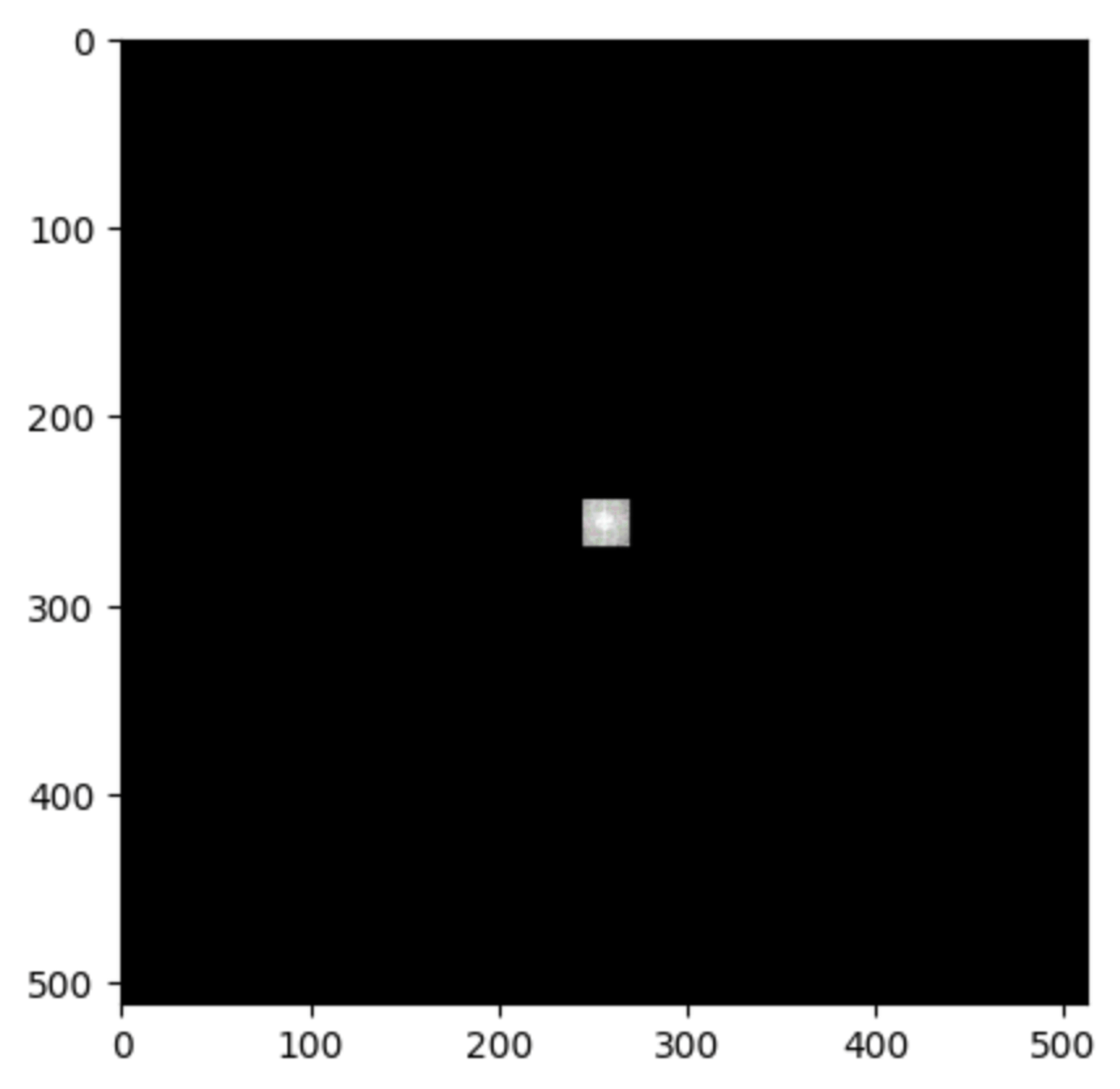
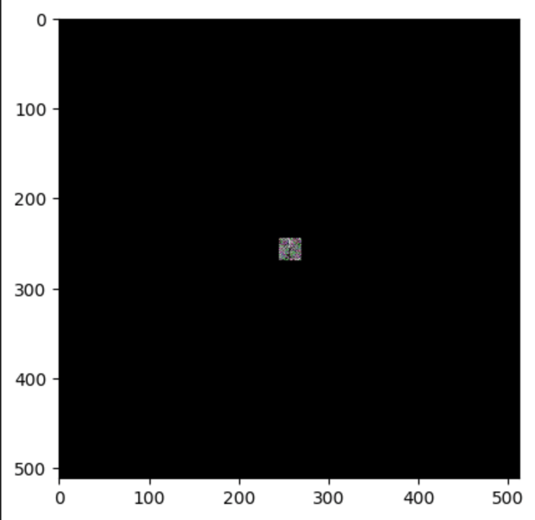
The center of the array corresponds to the lowest frequencies of the image, where the intensity of pixel values changes slowly as we move across the image. Low frequencies make up most of the information in the image that is really meaningful to us.
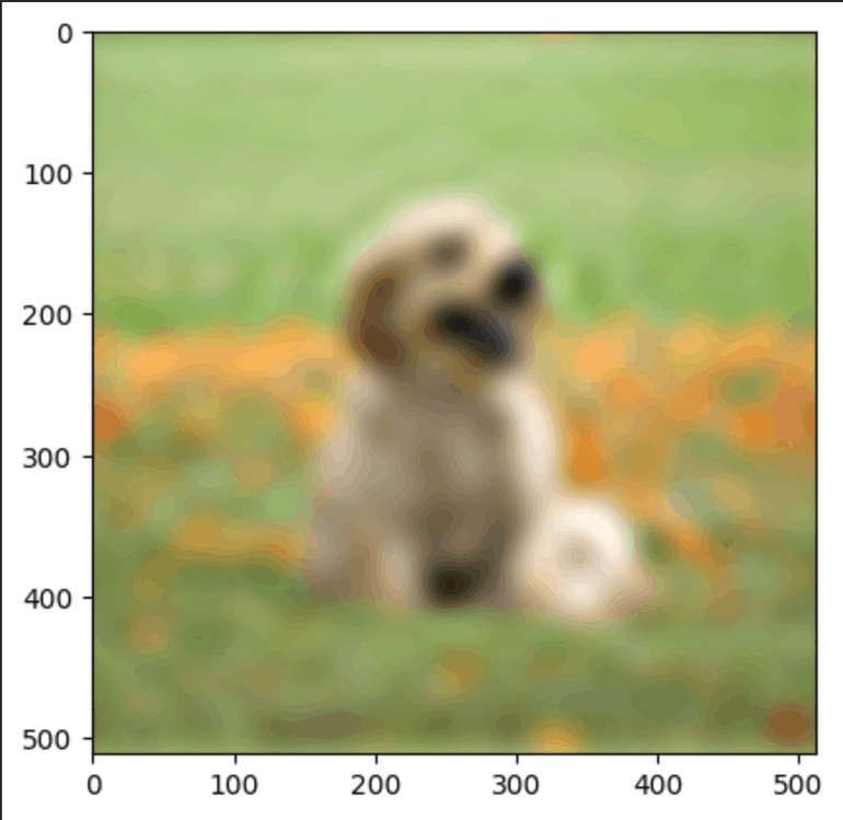
Look how much we lost here.
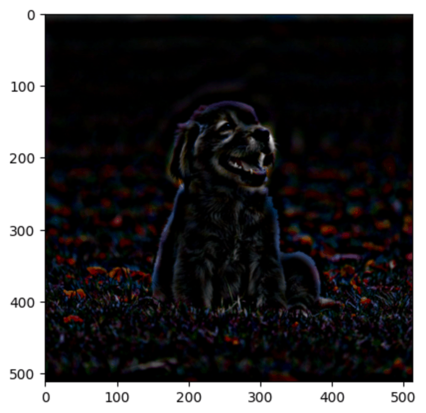
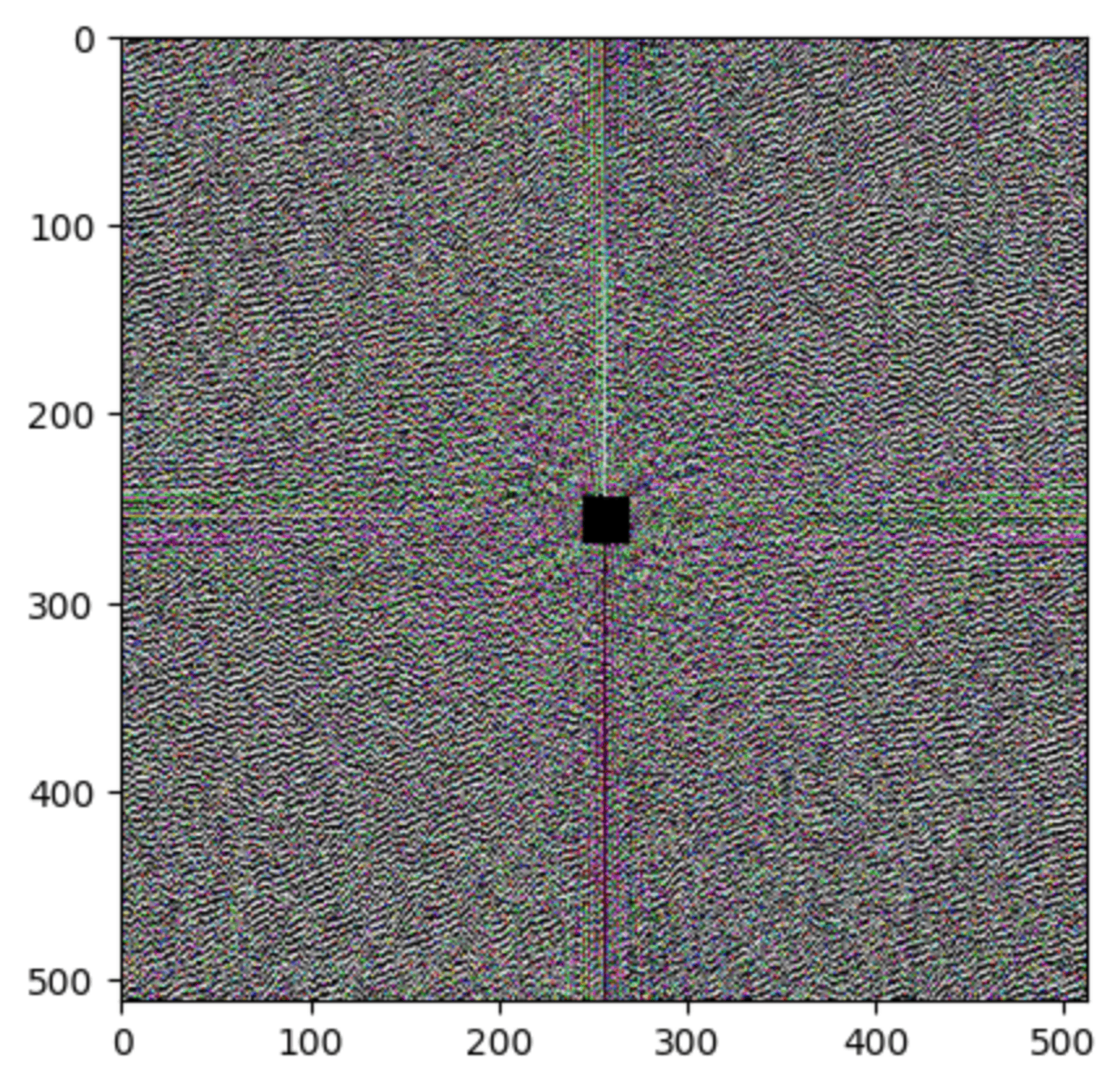
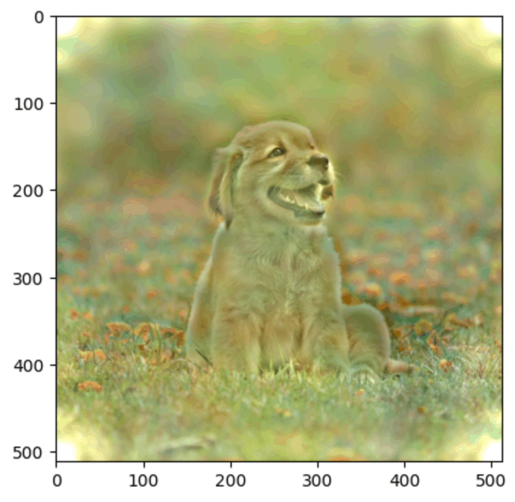
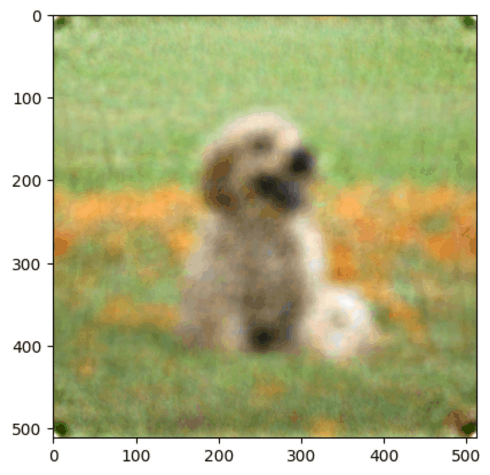
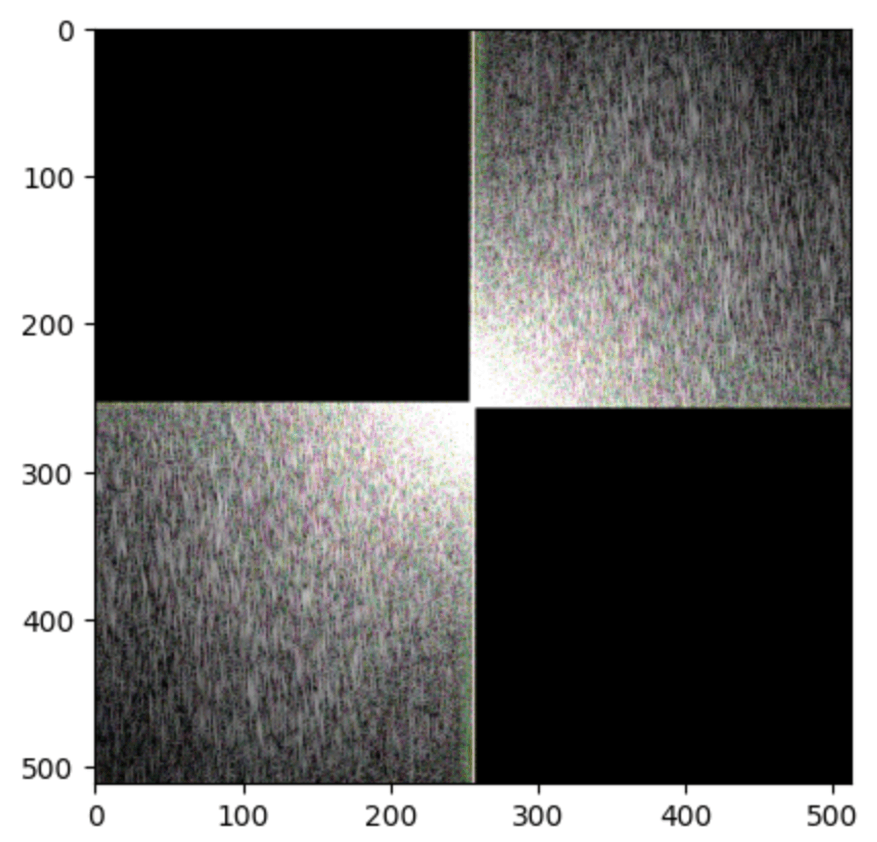
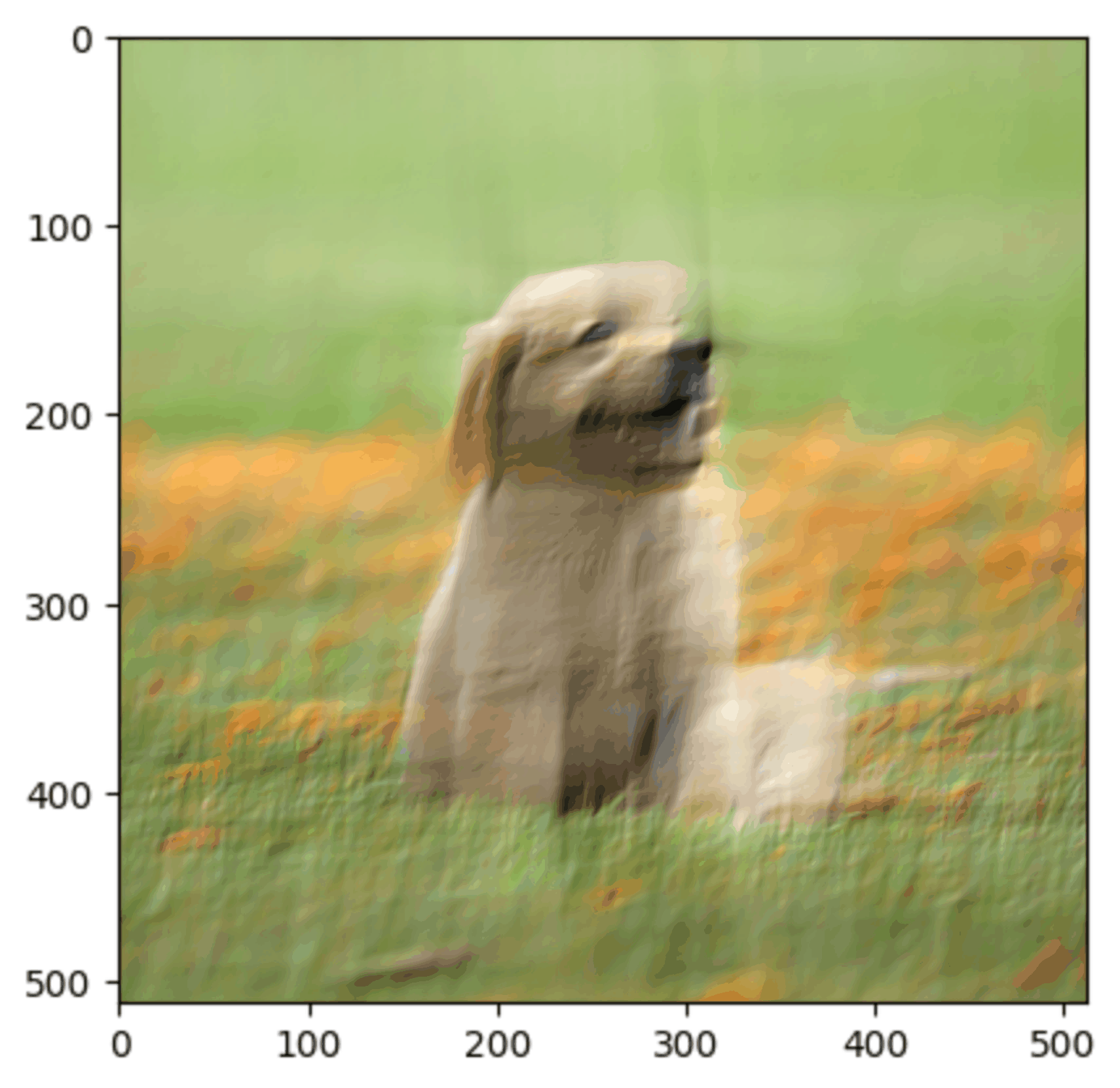
Here’s what happens when I zero out the inverse of the above
What I just did there acts as a High Pass Filter and a Low Pass Filter on the image respectively.
A High pass filter extracts only the higher frequencies of the image, points where pixel values change more rapidly.
Meanwhile a Low pass filter extracts only the lower frequencies of the image, causing a blur effect.
Here’s the same strategy performed to the phase information (in this case, for zeroing i’ll set the angle to 0)
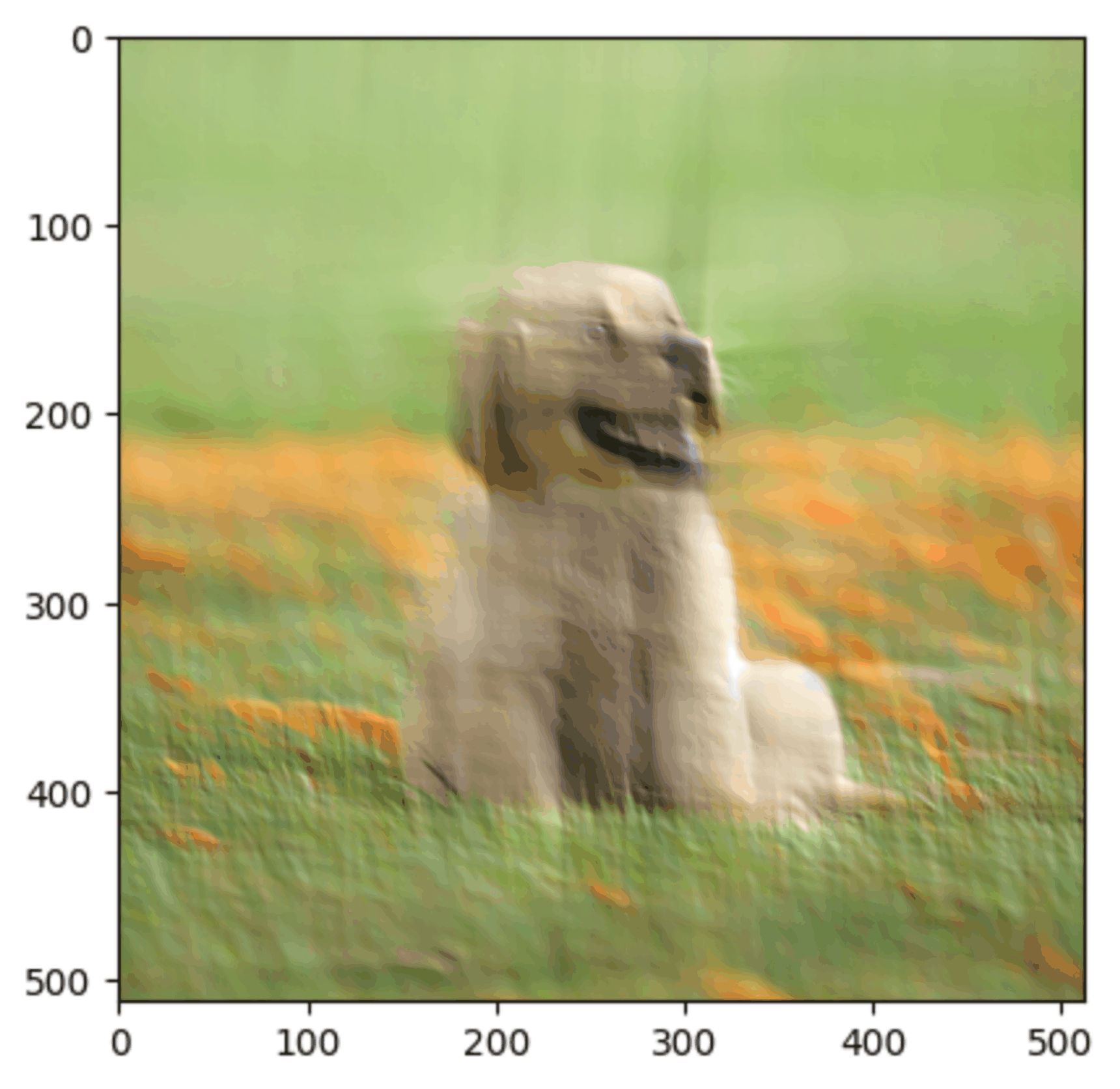
Now I want to give a sense of what happens when we zero out diagonals for the magnitude.
Not sure how well it can be seen here but there’s sort of a directional look of it. If you’ve ever messed around with certain tools in Photoshop like bevel or the texture stuff where it asks you to specify a global lighting direction, how this looks kinda reminds me of that.
To better visualize this effect, I wrote a function that will iteratively “build” an image by adding one frequency at a time to the image. Done at 64x64 because this can take a really long time.
perhaps you can see why this could make for an interesting generative model!
Diffusion Models From a Perspective of Frequencies
I recall several papers discussing how Diffusion models, when generating an image, first develop the lower frequencies of an image and then the higher frequencies later. I can’t find them at the moment, but I do have some of my own visuals to show why this is a fair way to think about it.
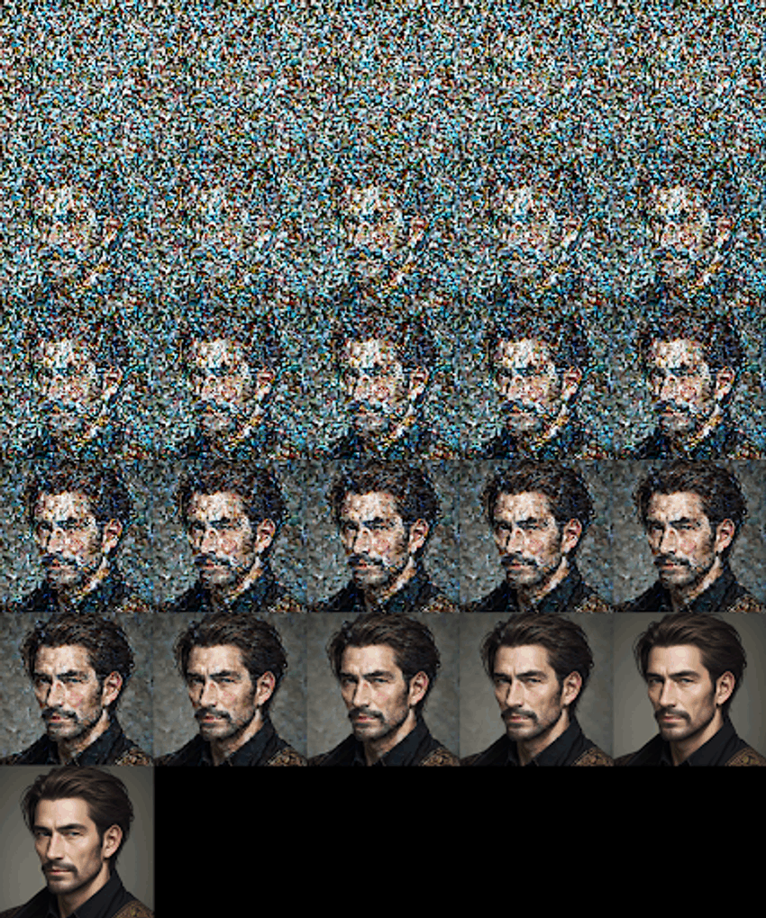
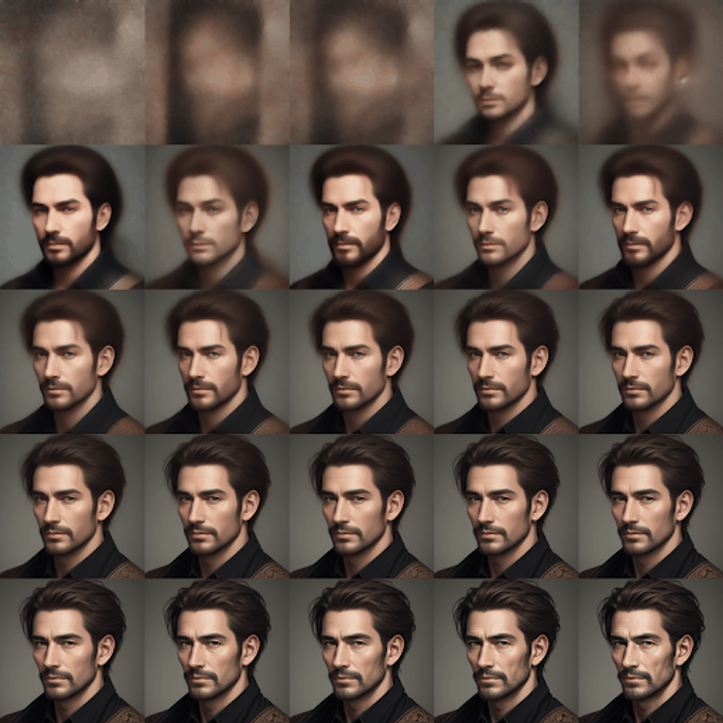
To start, let’s visualize the generation process of Stable Diffusion for a 25 step generation. Starting from latent noise and ending at the fully generated image.
Now what we can do, noting that the output of the model at every step is the prediction of noise that was added to the image, we can then subtract that noise to get a prediction of what the finalized image looks like as its still cooking.
Not so dissimilar to what we saw with the dog, we start off blurry and build up finer and finer details over the course of the generation.
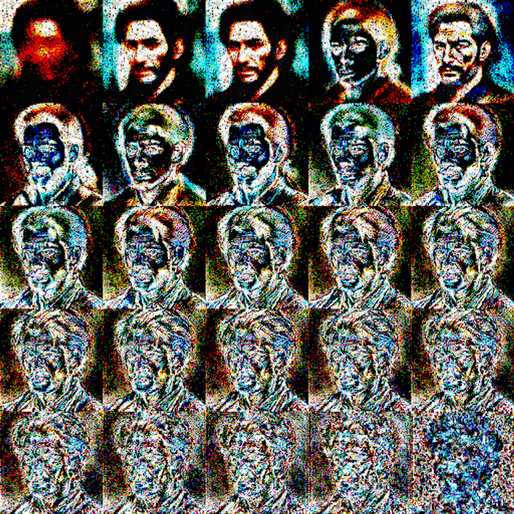
Additionally, to really show that a frequency is being “worked on” at a certain step, we can visualize the difference between the text-conditioned prediction and the unconditional prediction. This difference map indicates where the greatest effect of classifier-free-guidance occurs.
Now its a bit of a mess because we’re taking the difference between latents and this is kind of hard to map back to pixel space, but we can see the highest attended areas start off as coarser regions and move on to edges like eyebrows and face contours and then the really finer details like texture of the hair.
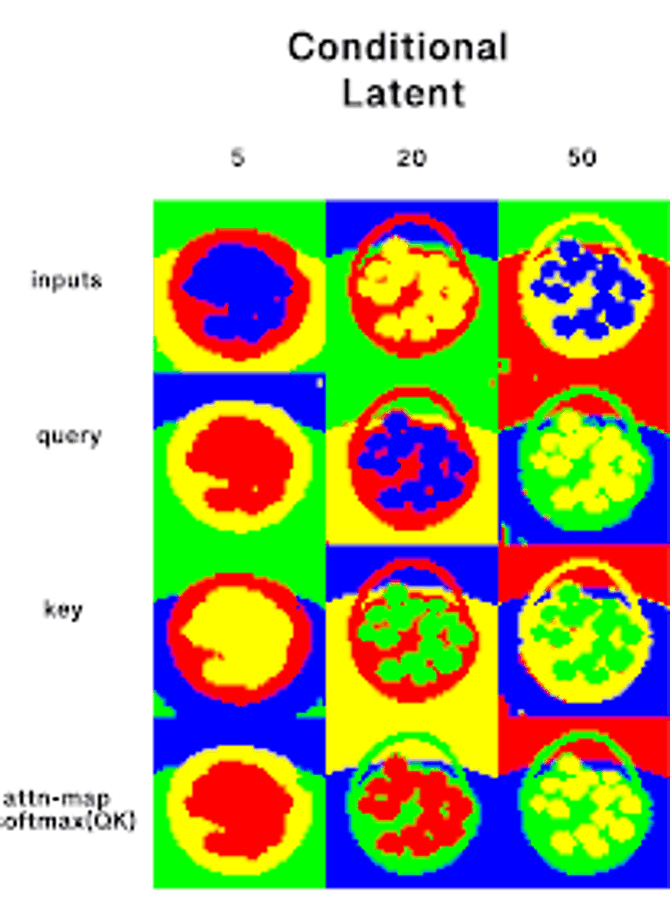
As a bonus, I ran a k-means clustering on latent features in the network across different timesteps. This was a picture of a basket of oranges. In early steps, we only really get the coarse structure of the image.
Also from Sander Dielman’s blog on diffusion which I highly reccomend, this graphic that shows how adding noise to an image can act as a low-pass-filter.
Also, not sure how to formulate it, but I think the way that you can apply a gaussian blur filter in the data space shares some similarities to how you convolve a gaussian with the image in probability space to add noise to it in terms of which frequencies are affect at different magnitudes?
Methods
Design
The model is a typical transformer decoder model:
1024 dim
12layers
16 heads
Allocated 512 of dims for mean prediction, 256 for covariance and 256 for mixture probabilities
Inputs
First normalized [0,1]
Take the 2D-FFT of the image followed by FFT-shift
Magnitude component is logarithm’ed to give nicer range values to work with
Two things to note about the resulting FFT when turning it into a sequence
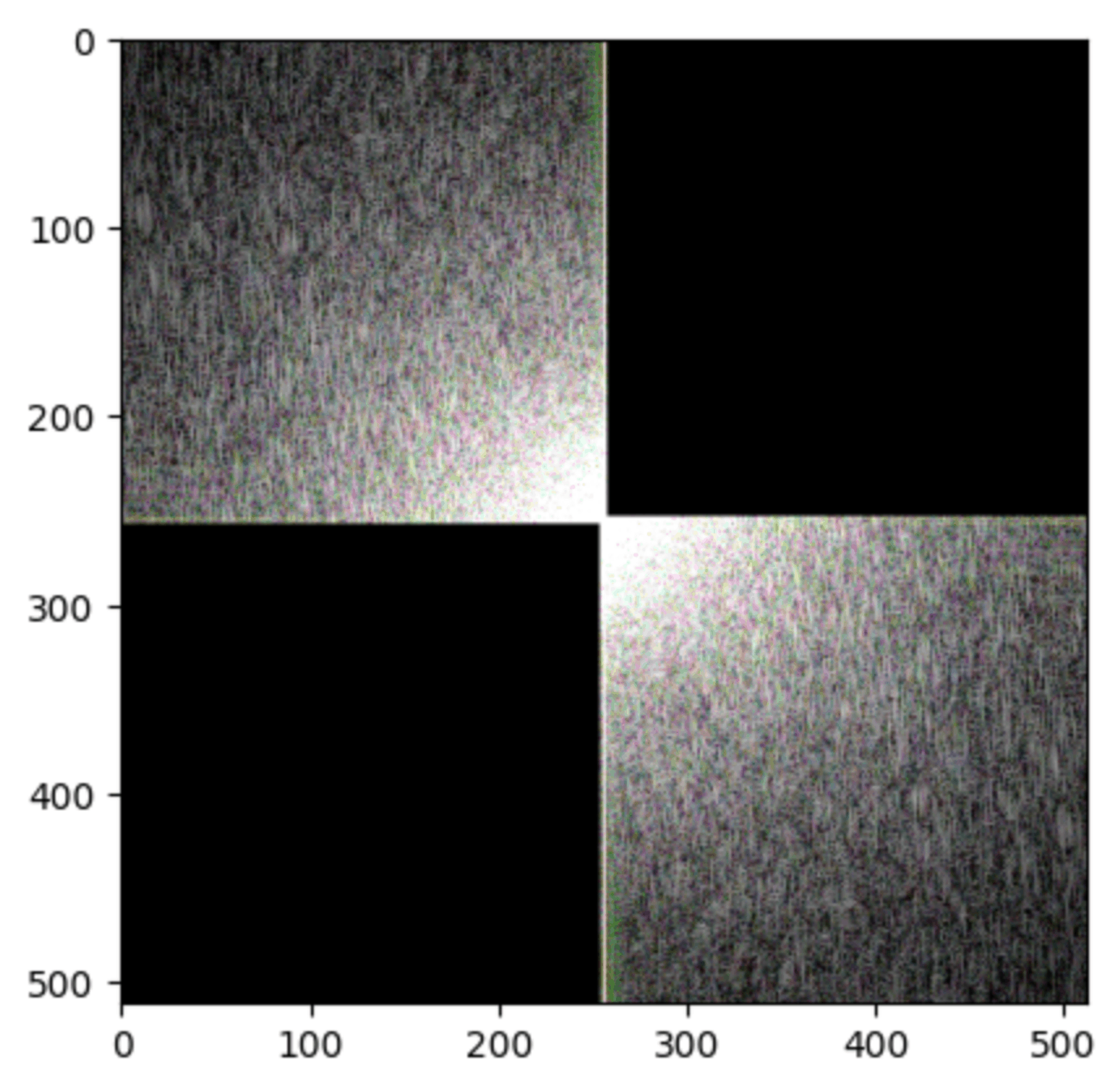
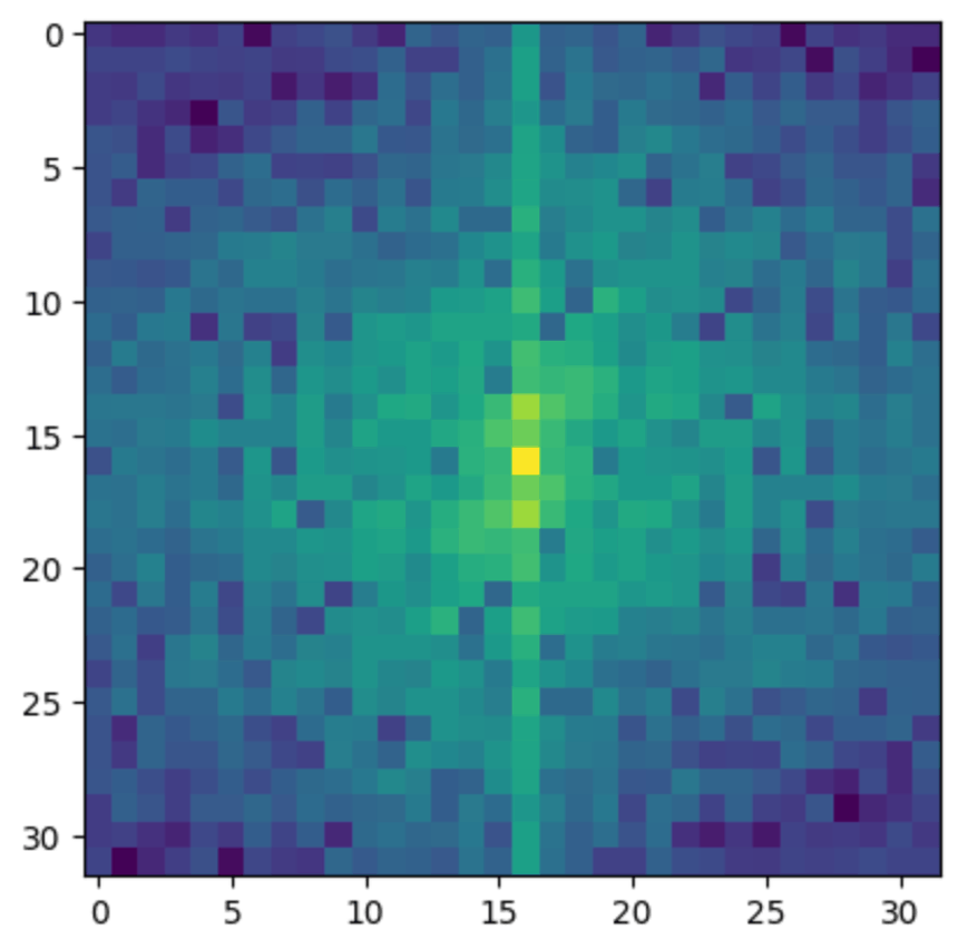
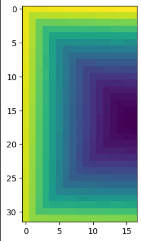
Firstly, you’ll notice that there’s a symmetry in the values, so we can get away with only taking half of what’s present
The right side is the left side rotated 180 degrees
To actually get the sequence, we’ll let the value in the center be first, then spiral around outward, which looks like this
When transforming back, we’ll duplicate the left side, rotate it 180 degrees and concatenate it.
I tried a few methods of embedding the data.
Quantization:
We’d discretize the range of values for phase and magnitude and give them each their own embedding table.
Incoming values would be clipped to their nearest value and embedded
This method also lends itself to predicting discrete values
Therefore, we’ll flatten our channels into the token dimension, such that we have
[R_mag0, G_mag0, B_mag0, R_phase0, G_phase0, B_phase0, R_mag1 …] x num_pixels
Fourier embedding - Continuous:
We use a Fourier embedding to project the coefficients to a higher dimension and then proceed with the rest of the network
In this case we can choose any kind of output shape, i.e. we could let one token be [R_mag, R_phase] … [G_mag, G_phase], but in most cases I let all 6 of the values corresponding to one pixel be the token
Losses
MSE
This sort of assumes that larger distance from the target point is proportionally worse, and doesn’t really acknowledge we can have multiple modes
not a great choice and doesn’t seem to work
Cross Entropy - quantized mode only
Typical cross entropy loss same as language models
Gaussian Mixture model log-probs (GMM)
set a number of gaussians we want as a hyperparameter
Have tried both assuming independence vs also outputting a covariance matrix, with the covariance option clearly winning
This makes sense as the values for R_mag for instance may be quite correlated with what we sample for B_mag
The output consists of the means, covariance matrix, and mixture probabilities.
Assuming we take the strategy of outputting all 6 values ([R_mag, G_mag, B_mag, R_phase, G_phase, B_phase]), the total number of output elements we have is:
6 means X num_gaussians
6x6 covariance matrix X num_gaussians
6 mixture_probs X num_gaussians
The loss when using covariance is a bit fragile, the covariance matrix calculations require float32 precision to work in any capacity and the outputted values from the NN need to be positive semi-definite.
The gradient norm also ends up being very large and chaotic
When sampling, we can sort of think of this as being pretty similar to the kind of sampling done for language models
Softmax the mixture probabilities
Use that to sample a corresponding mean
only differs once we add a bit of noise through either predicted standard deviation or covariance
Transform back into pixel space and take MSE or LPIPS loss there
Have not tried this, the series of transforms I have for going from 2d array of coefficients to flattened sequence is currently not differentiable.
A note on Gaussian Mixture Models vs working with discrete options as in the vocabulary of language models:
These two approaches are kind of similar when your discrete options are discretizing a continuous space.
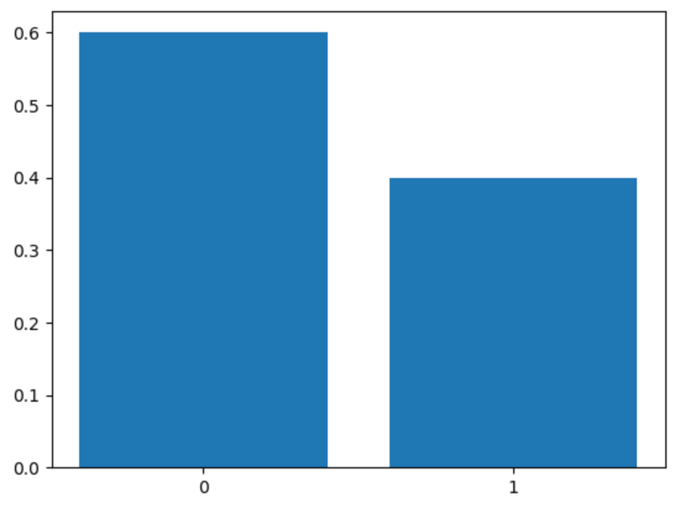
Here’s what it looks like when our discrete choices are 0 and 1, with 60% of the mass on 0 and 40% on 1
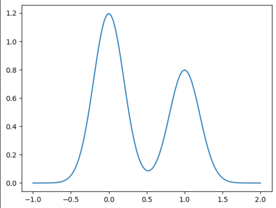
Alternatively, here’s what a gaussian mixture model looks like when we have two gaussians parameterized by means of 0,1, stds of 0.2,0.2 and mixture probabilities 0.6 and 0.4
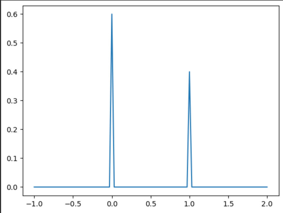
We can take a different perspective of the first approach as being a gaussian mixture model but with std approaching 0, (not normalized to have area of 1 under curve)
Other losses
Angle Loss
Because angle is constricted to the range of [-pi, +pi], and keeping in mind that -pi and +pi are equivalent, we need to be clever in how we compute the loss for it. i.e. if the target is 3.10 and we predict -3.12, the GMM loss or MSE would be very large, and wrongfully so.
When sampling we can use a modulo such that a value of +3.28 for instance will become -3.00
I also added an additional loss at a low weight that penalizes predictions >3.14 or < -3.14
When computing the loss, take the difference between the modulo’ed version and the original and take the lower of the two
we can use torch.where to have a differentiable modulo.
Variance Loss
a very low weight loss to encourage low variance in the predicted gaussians
Not really sure how useful it is, but I put it in as I was concerned that the randomness could cause an accumulation of errors between steps and maybe penalizing variance a bit could help.
Results
Quantized Method
200 epochs on flowers102
8.0e-5 lr on linear decay
batch size 40
warmup steps: 250
vocab_size: 8192 — torch.linspace(-7.5, 7.5, vocab_size) this is sufficient to capture full range of values
Conditions are pretty similar to the single-variate gmm, but this time we have a fixed vocabulary, of quantized values.
It’s sort of as if we were to cut out the means and stds and only predict the mixture probabilities, mapping them as position indices to our fixed set of values.
However, I feel its a pretty awkward and inefficient approach. There’s no design that sort of tells it that if you predict 4.0001 vs 4.0002 they’re basically the same (assuming they get clipped to different values)
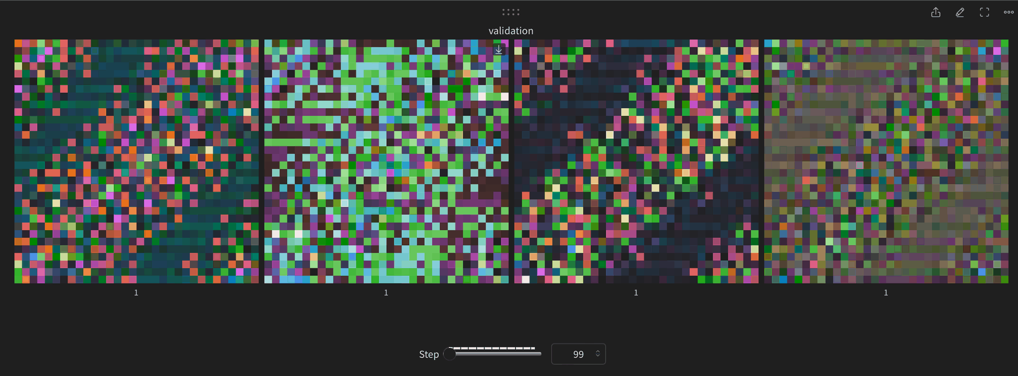
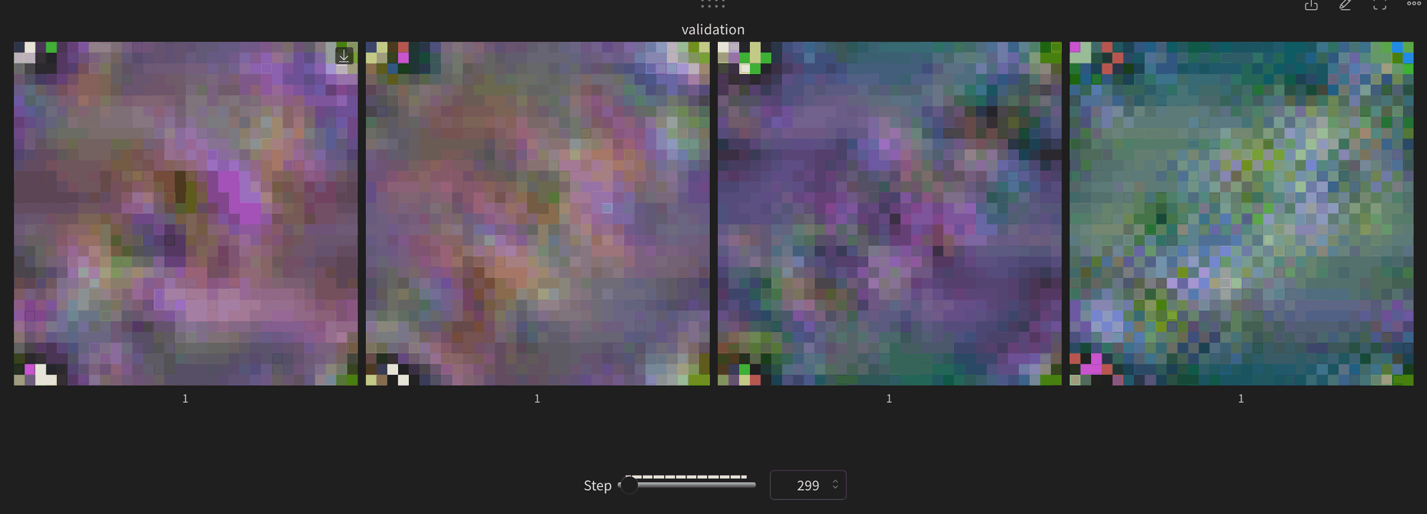
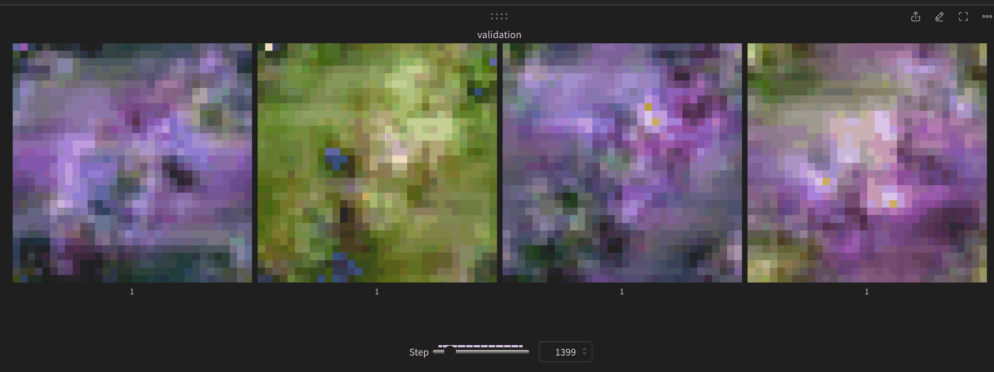
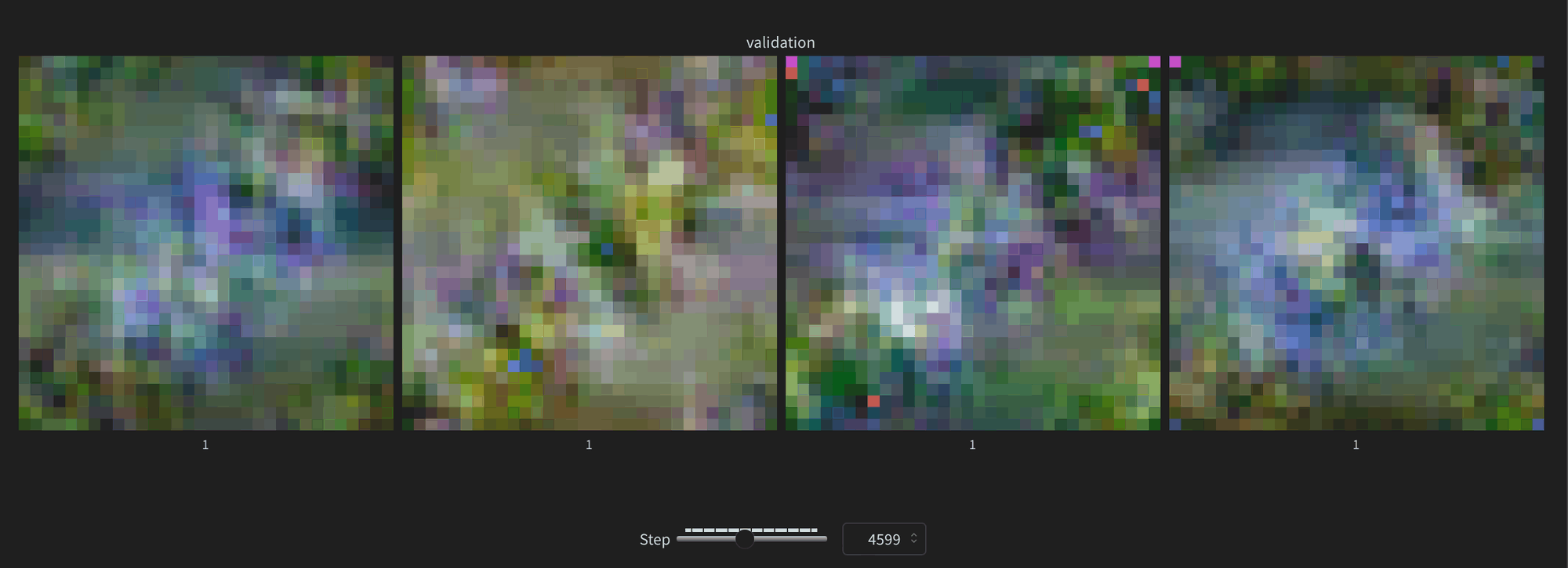
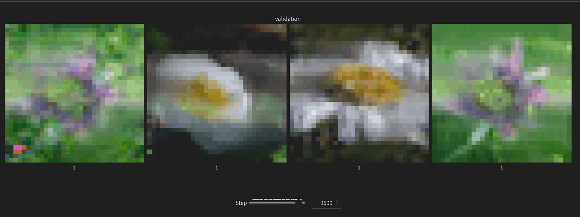
The progression of samples are pretty cool
andddd we’re overfitting, although i also realized i set topk-sampling to 10
net result is pretty cool nonetheless
Multivariate Gaussian Mixture Model - predicting all 6 channels at once
200 epochs on flowers102 (cut halfway through as it wasn’t looking promising)
1.5e-4 lr on linear decay
batch size 256
warmup steps: 250
Not great results with this in terms of visual results, although I’m wondering if it did otherwise work and I may just be sampling incorrectly?
This method is a bit unstable in the computations done for the covariance matrix, but its nice because our sequences are only ~500 tokens long
If we unroll the channels into tokens we have ~3000 long sequences.
I may try this method again as a single variate gaussian mixture model, just as I think it makes sense to properly acknowledge the continuous space we’re working with.
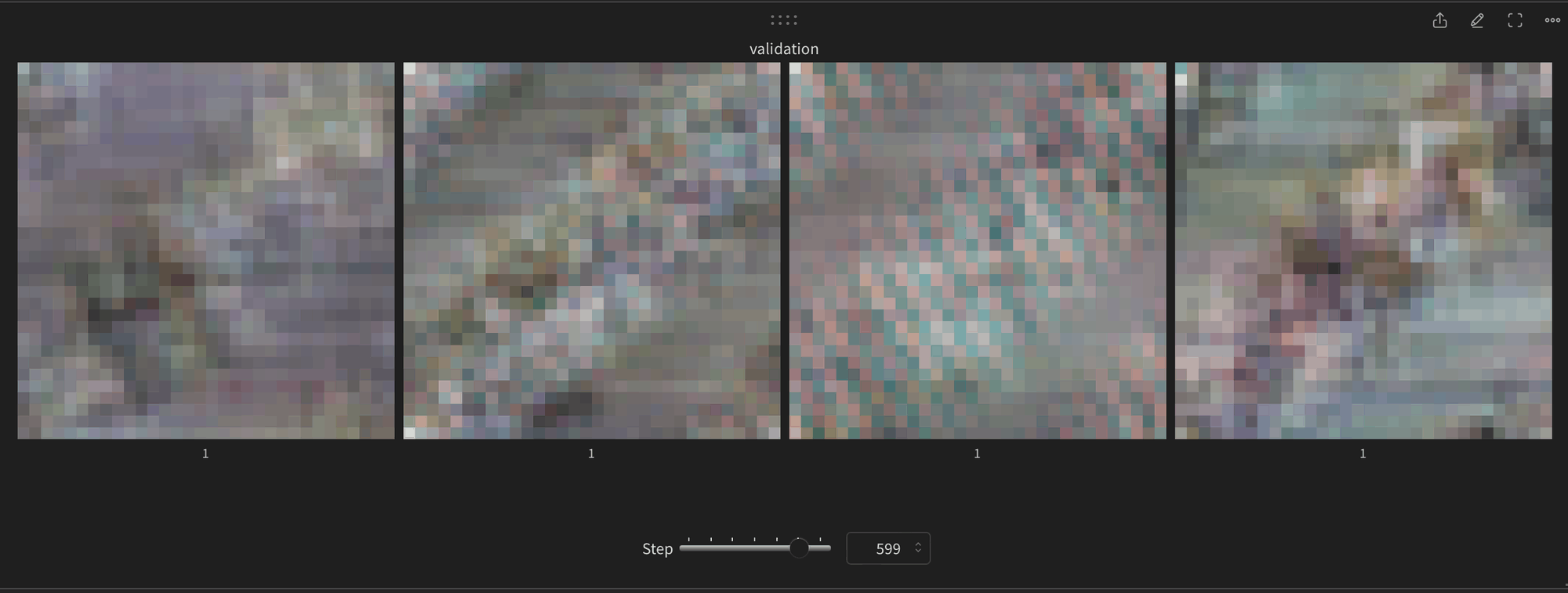
600 steps in
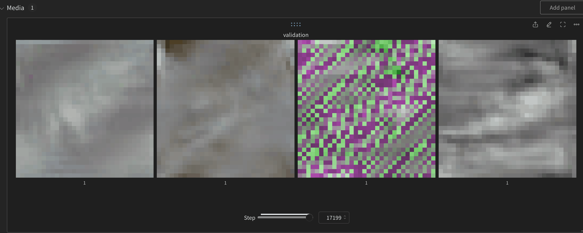
17000 steps in still nothing exciting to look at, as well as some occasional artifacts
I took a sample of the predicted means at the 0th position and 100th position and they do appear properly diverse, i.e. not collapsing to single mode.
Click to view
JavaScript
Copy
sample of means at pos 0: tensor([[ 3.5156, 3.2812, 3.1875, 1.9766, -2.5781, 2.4844],
[ 4.2812, 2.8750, 3.9688, -0.2871, 0.0413, -0.3184],
[ 3.1875, 3.2812, 3.2188, -1.5078, -2.0469, -1.6484],
[ 3.6875, 3.7656, 3.7188, -1.5469, -1.9531, -1.6250],
[ 4.0625, 4.0938, 4.1250, -2.7500, 2.9844, -2.9531],
[ 4.8750, 4.6250, 4.8438, -0.6758, -0.8438, -0.6836],
[ 3.6250, 3.5625, 3.4219, -0.0106, 0.3320, 0.0542],
[ 4.6250, 4.2188, 4.5625, -0.5742, -0.7266, -0.5625],
[ 3.8438, 4.0312, 3.9531, -0.0317, 0.1514, 0.0500],
[ 4.5000, 4.4688, 4.5312, -2.0469, -2.1094, -2.0781]],
device='cuda:0', requires_grad=True)
sample of means at pos 100: tensor([[ 0.5195, 0.1602, 0.0962, 2.5781, -2.8750, 2.7812],
[ 0.3691, -0.8203, -0.0933, 1.5078, 0.8359, 1.2109],
[-0.1631, 0.0845, -0.1064, -2.5156, -1.8750, -1.8984],
[ 0.4590, 0.6680, 0.5352, -2.3438, -1.9531, -2.0312],
[ 1.2188, 1.1328, 1.1328, -3.0000, 3.0938, -3.0469],
[ 1.7109, 1.6797, 1.7266, 0.4668, 0.3477, 0.3965],
[-0.1465, 0.1245, 0.1123, 0.4160, -0.3672, -0.1221],
[ 1.1250, 1.0312, 1.1250, 0.9023, 0.6797, 0.7461],
[ 0.5508, 0.8555, 0.8242, -0.3750, -0.6211, -0.4941],
[ 1.6875, 1.7422, 1.7109, -2.3906, -2.2969, -2.2969]],
device='cuda:0', requires_grad=True)
The stds, (diagonal of covariance matrix) appear pretty small, but I don’t think this is necessarily strange, especially since we’re operating on a log-scale. (Although now this is making me wonder if there’s a better kind of normalization than log-scale)
Click to view
JavaScript
Copy
sample of stds at pos 0: tensor([[0.2788, 0.5299, 0.3848, 0.3196, 0.2106, 0.2667],
[0.2791, 0.7909, 0.3204, 0.9700, 3.0202, 0.9190],
[0.4067, 0.4412, 0.4508, 0.5815, 0.5721, 0.4568],
[0.4309, 0.3491, 0.3600, 0.5438, 0.4441, 0.4462],
[0.3267, 0.3051, 0.2784, 0.0512, 0.0200, 0.0154],
[0.0907, 0.1105, 0.0924, 0.4867, 0.5589, 0.4974],
[0.3192, 0.4427, 0.3619, 1.2977, 1.6520, 1.0248],
[0.1302, 0.1819, 0.1438, 0.6244, 0.8456, 0.6389],
[0.3105, 0.2957, 0.3021, 1.1548, 1.1696, 1.0735],
[0.1153, 0.1027, 0.0975, 0.2976, 0.2577, 0.2549]], device='cuda:0')
sample of stds at pos 100: tensor([[0.1480, 0.2441, 0.1908, 0.1083, 0.0472, 0.0661],
[0.1115, 0.3616, 0.1108, 0.4035, 1.7481, 0.6148],
[0.2030, 0.2295, 0.1712, 0.2228, 0.3063, 0.2521],
[0.1261, 0.0838, 0.0768, 0.2831, 0.2975, 0.3075],
[0.1713, 0.2517, 0.2536, 0.0117, 0.0073, 0.0040],
[0.0384, 0.0415, 0.0342, 0.5352, 0.5737, 0.5300],
[0.1866, 0.1773, 0.0994, 0.9298, 0.7113, 0.5486],
[0.0509, 0.0638, 0.0410, 0.6454, 0.7859, 0.6817],
[0.1120, 0.0631, 0.0541, 0.9465, 0.6103, 0.6261],
[0.0636, 0.0579, 0.0577, 0.2543, 0.2262, 0.2355]], device='cuda:0')
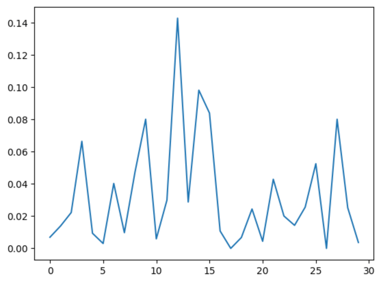
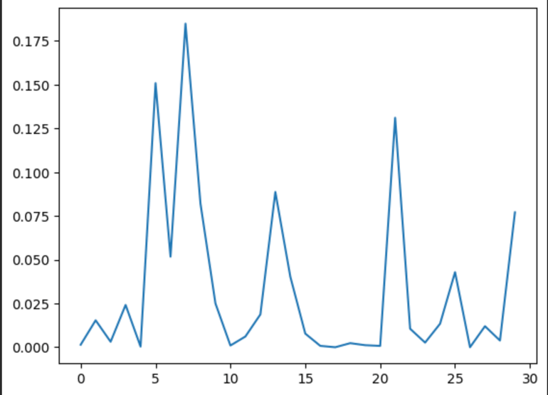
Mixture probabilities at position 0 and 100 respectively, perhaps a bit less peaked than I was expecting
Other stats
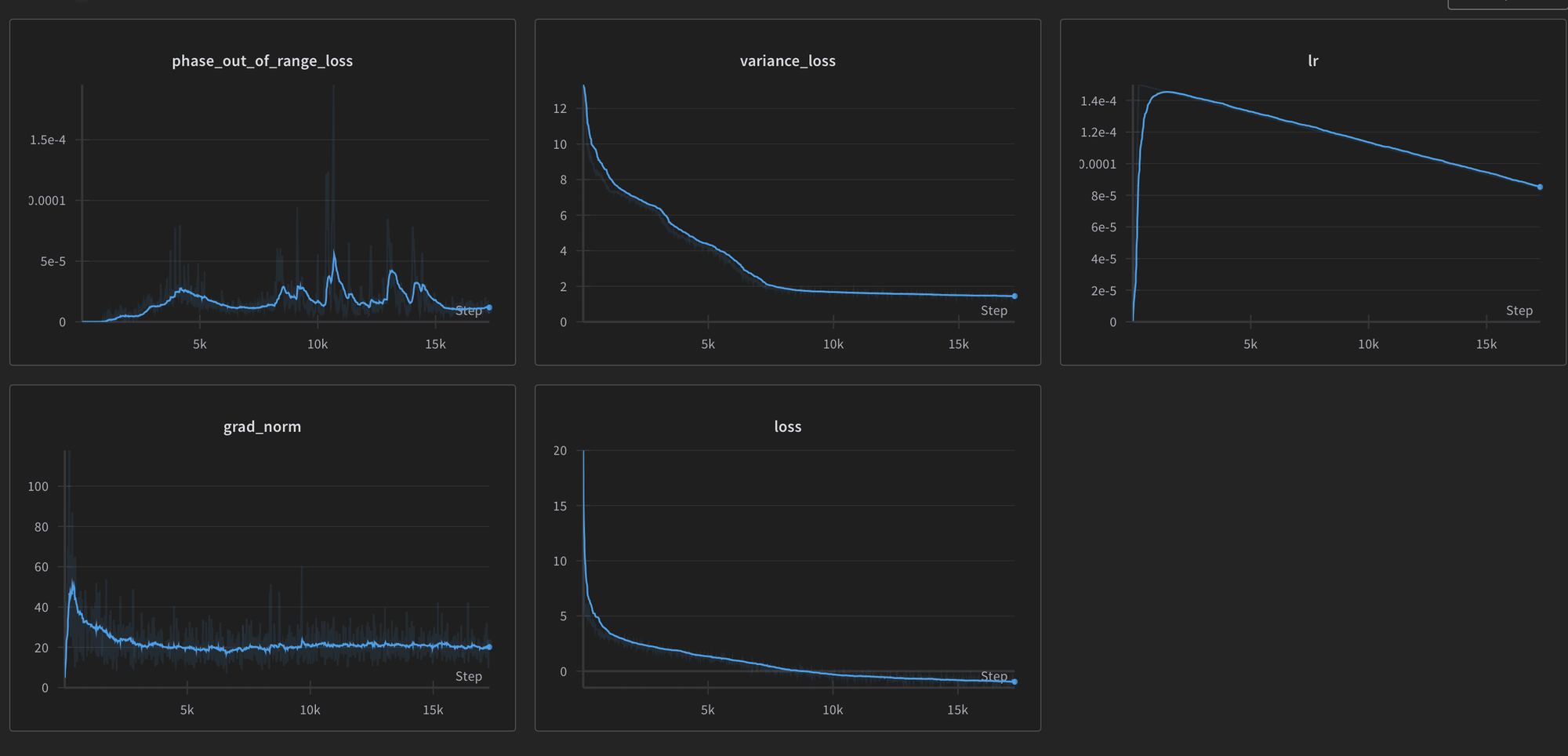
Notice that the loss actually goes negative
I freaked out initially and halted the training thinking my loss function was incorrect, it turns out if the covariance matrix is quite small and the error is small, this is possible.
It just matters that the total PDF can integrate to 1, we can have points of mass > 1.0
Single-variate gaussian mixture model
200 epochs on flowers102
8.0e-5 lr on linear decay
batch size 40
warmup steps: 250
We flatten all the channels, which brings us from 544 tokens to 3264, because of this 6x fold increase in sequence length and thus 36x increase in attention complexity, had to drop down the batch size quite a bit.
By doing this though, we can avoid having to calculate a covariance matrix. Instead now, the covariance is implicitly captured by the neural network and is reflected in the conditional probabilities when we sample the next channel.
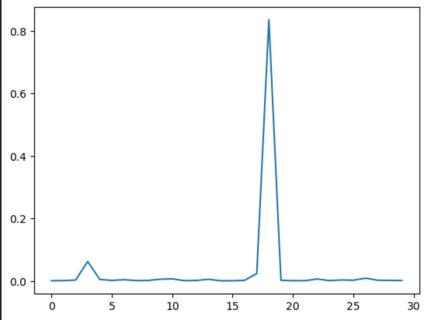
First thing to notice is that the mixture probs are way more peaked, this is seen even as early as the 400th step
JavaScript
Copy
@misc{smith2024,
author = {Smith, Ethan},
title = {Mimicking Diffusion by Sequencing Frequency Coefficients},
url = {https://sweet-hall-e72.notion.site/Mimicking-Diffusion-Models-by-Sequencing-Frequency-Coefficients-8e5a60e876d640c390369627d55330b1?pvs=4},
year = {2024}
}

